3D Scatter Plot (Python)

🤖 AI Skill — Download the Bizard unified skill for your AI assistant ⬇️ Download Skill ZIP

🔌 MCP Server — Let AI agents (Claude Code, Cursor, …) query Bizard live: claude mcp add bizard -- npx @openbiox/bizard-mcp — or the free hosted instance (no install, faster from mainland China): claude mcp add --transport http bizard http://biotree.top:38123/bizard-mcp/mcp 📖 MCP Docs

📖 Cite Bizard — if Bizard helps your research, please cite: Li, K., Zheng, H., Huang, K., et al. (2026). Bizard: A Community-Driven Platform for Accelerating and Enhancing Biomedical Data Visualization. iMetaMed, e70038. 🔗 DOI / BibTeX

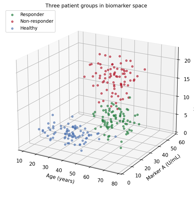
The Python counterpart of 3D Scatter — a 3D scatter places each subject at \((x, y, z)\) coordinates of three quantitative variables, adding one biomarker dimension to the classic 2D plot. In translational research it helps when group separation genuinely lives in three variables (age x marker x marker, cell size x granularity x intensity) and a static 2D projection visibly flattens it [1].

matplotlib’s mplot3d renders the projection [2]. Two properties make 3D scatter plots easy to misread: the view angle decides which clusters hide behind which, and depth is encoded only by size/alpha shading — a printed 3D plot is a single fixed projection of a 3D object. Both should be treated as parameters to report, like a model.

This tutorial covers two workflows:

1. A default-view 3D scatter of three patient groups;
2. A rotation panel showing how the same data changes its story.

Example

Setup

• System Requirements: Cross-platform (Linux/MacOS/Windows)
• Programming Language: Python
• Dependencies: matplotlib, numpy

import matplotlib.pyplot as plt
import numpy as np
from mpl_toolkits.mplot3d import Axes3D  # noqa: F401 (registers 3d projection)

Data Preparation

We simulate 240 subjects in three groups with distinct (age, marker A, marker B) profiles: responders are older with mid-range markers, non-responders have the highest markers, healthy donors the lowest. The separation direction is chosen so some viewpoints separate the groups and others collapse them.

rng = np.random.default_rng(21)
groups = {
    "Responder":     (np.array([60, 25, 8]),  np.array([8, 6, 2.2]),
                      "#1B7837"),
    "Non-responder": (np.array([48, 40, 15]), np.array([9, 7, 3.0]),
                      "#B2182B"),
    "Healthy":       (np.array([35, 12, 4]),  np.array([10, 4, 1.4]),
                      "#4C72B0"),
}
n_per = 80
data = []
for g, (mu, sd, color) in groups.items():
    xyz = np.column_stack([rng.normal(m, s, n_per)
                           for m, s in zip(mu, sd)])
    data.append((g, xyz, color))

def draw(ax, elev, azim, title):
    for g, xyz, color in data:
        ax.scatter(xyz[:, 0], xyz[:, 1], xyz[:, 2], s=14, alpha=0.6,
                   color=color, label=g, depthshade=True)
    ax.set_xlabel("Age (years)")
    ax.set_ylabel("Marker A (U/mL)")
    ax.set_zlabel("Marker B (ng/mL)")
    ax.view_init(elev=elev, azim=azim)
    ax.set_title(title, fontsize=10, pad=0)
    ax.set_box_aspect((1, 1, 0.8))

Visualization

1. Default View

fig = plt.figure(figsize=(7.5, 5.6))
ax = fig.add_subplot(111, projection="3d")
draw(ax, elev=20, azim=-60,
     title="Three patient groups in biomarker space")
ax.legend(loc="upper left", fontsize=9)
fig.tight_layout()
plt.show()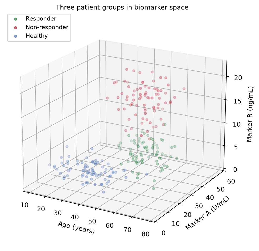

Figure 1: Three patient groups in biomarker space at elev=20, azim=-60: the groups occupy distinct regions of the 3D volume.

2. Rotation Panel

fig = plt.figure(figsize=(11.5, 4.8))
for i, (elev, azim, title) in enumerate([
        (20, -60, "View A (elev=20, azim=-60): groups look separable"),
        (2, 55, "View B (elev=2, azim=55): edge-on view obscures depth")]):
    ax = fig.add_subplot(1, 2, i + 1, projection="3d")
    draw(ax, elev=elev, azim=azim, title=title)
fig.suptitle("One dataset, two stories: rotation changes the reading",
             y=1.0)
fig.tight_layout()
plt.show()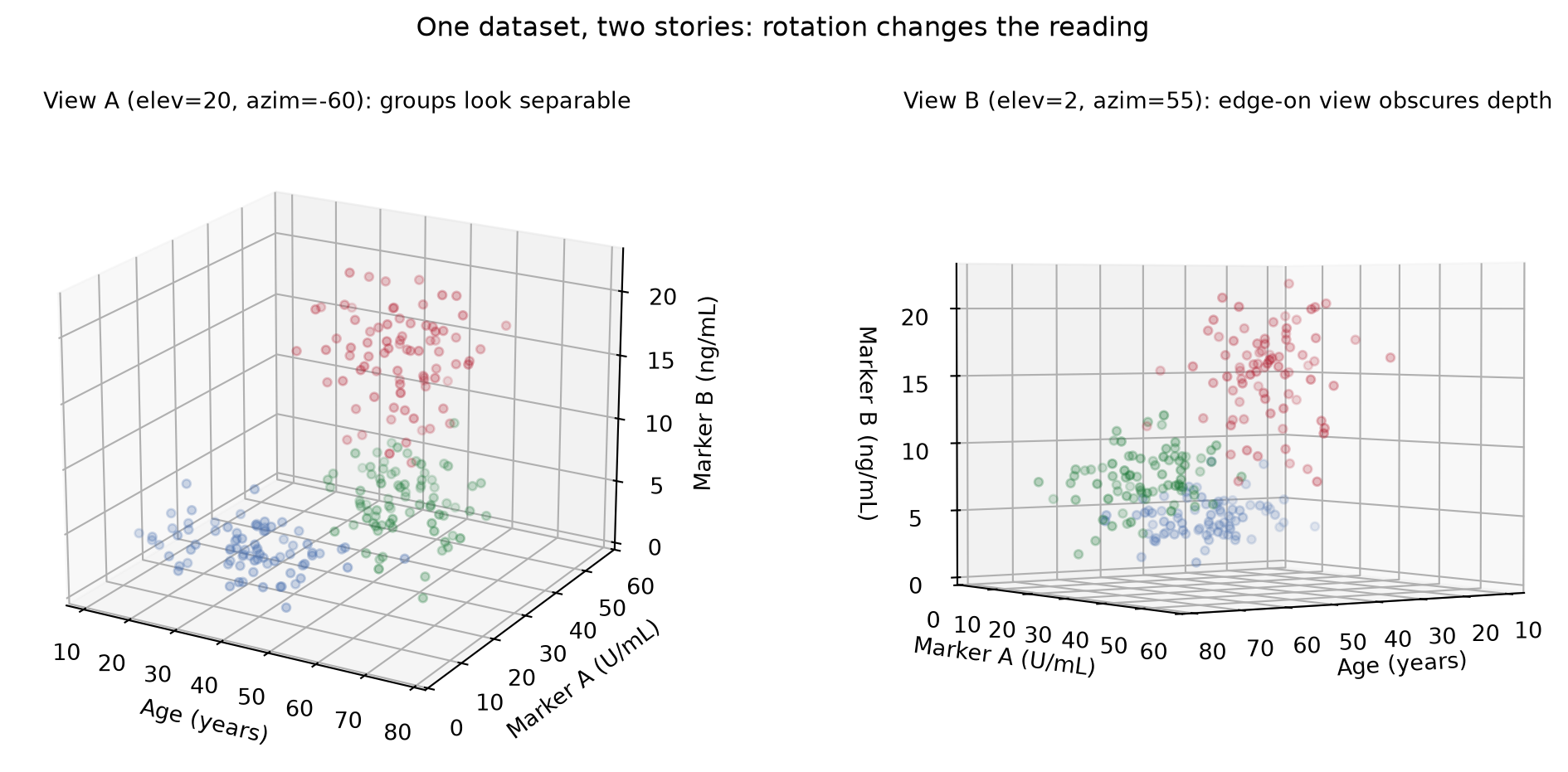

Figure 2: The same dataset from two viewpoints: the separability reading at left is not available edge-on at right, where depth order and the reversed axis direction become hard to judge.

TipPractice tips

• Report elev/azim in the caption when a claim depends on the viewpoint; a reviewer cannot otherwise reproduce your separation.
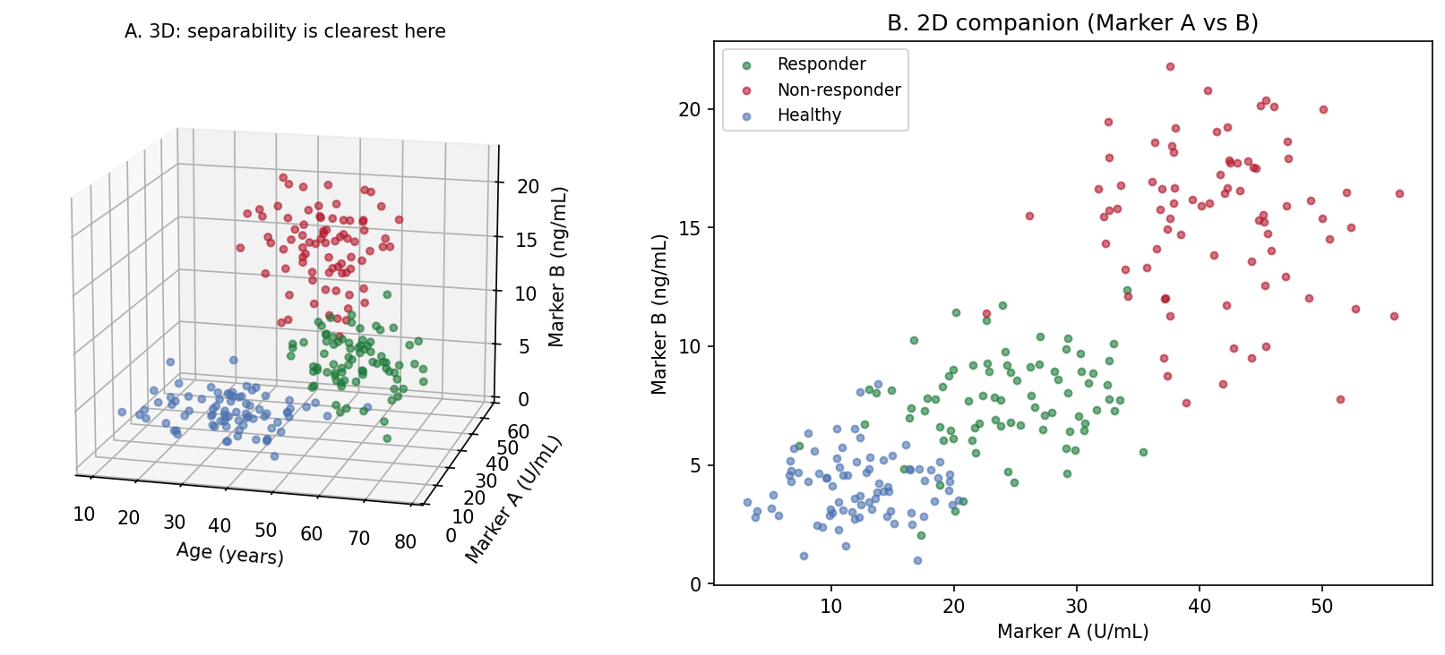
• alpha + depthshade only suggest depth — points still overplot. Lower alpha and smaller markers reduce false occlusion judgments.
• Prefer 2D panels of the variable pairs (Application panel B) for any quantitative comparison; use the 3D view to motivate them.
• Set ax.set_box_aspect() to a physically meaningful ratio, or a 3x range axis will visually dominate a 1x range axis.
• Interactive rotation (notebook %matplotlib widget, plotly Scatter3d) is for exploration; export the chosen angle for publication.

Application

The publication pairing places the chosen 3D view (A) next to its strongest 2D projection (B): the 3D panel motivates the three-group structure, and the 2D panel carries the readable, quantitative comparison that the paper’s statistics refer to.

Reference

[1] Li J, Martens JB. Judging correlation from scatterplots: an evaluation of 3D visualizations. IEEE Trans Vis Comput Graph. 2010;16(6):1027-1036.

[2] Hunter JD. Matplotlib: a 2D graphics environment. Comput Sci Eng. 2007;9(3):90-95. doi:10.1109/MCSE.2007.55