# Installing necessary packages
if (!requireNamespace("ggplot2", quietly = TRUE)) {
  install.packages("ggplot2")
}
if (!requireNamespace("dplyr", quietly = TRUE)) {
  install.packages("dplyr")
}
if (!requireNamespace("tidyr", quietly = TRUE)) {
  install.packages("tidyr")
}
if (!requireNamespace("corrplot", quietly = TRUE)) {
  install.packages("corrplot")
}
if (!requireNamespace("ComplexHeatmap", quietly = TRUE)) {
  BiocManager::install("ComplexHeatmap")
}

# Load packages
library(ggplot2)
library(dplyr)
library(tidyr)
library(corrplot)
library(ComplexHeatmap)Immune Subtype Plot
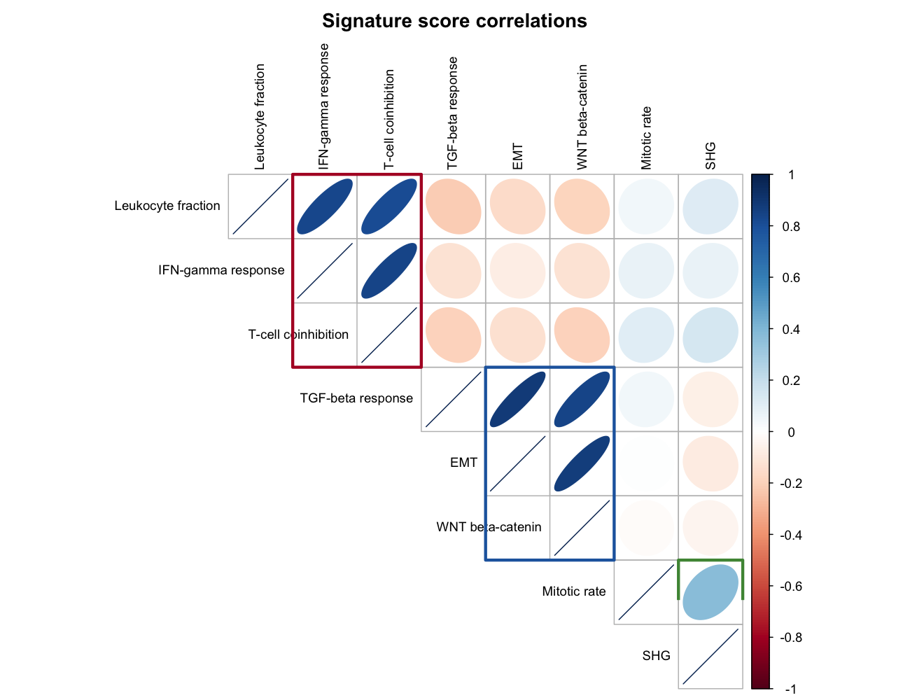
Clustering tumour samples by immune-infiltration signature scores is how the pan-cancer immune subtypes (C1–C6) of the reference paper were defined [1]: signature scores are correlated pairwise, modules of co-varying signatures are boxed, and samples are then clustered by the scores into subtypes whose score distributions characterise them. This tutorial reproduces that layout on simulated data: a module-structured correlation heatmap, sample clustering into subtypes, and the per-subtype score distributions that justify the naming.
Example
Setup
System Requirements: Cross-platform (Linux/MacOS/Windows)
Programming Language: R
Dependent packages:
ggplot2;dplyr;tidyr;corrplot;ComplexHeatmap
sessioninfo::session_info("attached")─ Session info ───────────────────────────────────────────────────────────────
setting value
version R version 4.6.2 (2026-10-29)
os Ubuntu 26.04.1 LTS
system x86_64, linux-gnu
ui X11
language (EN)
collate C.UTF-8
ctype C.UTF-8
tz UTC
date 2026-11-05
pandoc 3.7.0.2 @ /usr/bin/ (via rmarkdown)
quarto 1.11.9 @ /usr/local/bin/quarto
─ Packages ───────────────────────────────────────────────────────────────────
! package * version date (UTC) lib source
P ComplexHeatmap * 2.28.0 2026-04-28 [?] Bioconductor 3.23 (R 4.6.2)
P corrplot * 0.95 2024-10-14 [?] RSPM
P dplyr * 1.2.1 2026-04-03 [?] RSPM
P ggplot2 * 4.0.3.9000 2026-11-03 [?] Github (tidyverse/ggplot2@b638d65)
P tidyr * 1.3.2 2025-12-19 [?] RSPM
[1] /home/runner/.cache/R/renv/library/Bizard-5140bdc6/linux-ubuntu-resolute/R-4.6/x86_64-pc-linux-gnu
[2] /home/runner/work/_temp/Library
[3] /opt/R/4.6.2/lib/R/library
* ── Packages attached to the search path.
P ── Loaded and on-disk path mismatch.
──────────────────────────────────────────────────────────────────────────────Data Preparation
We simulate signature scores for 90 samples across 8 immune signatures, planted with three correlated modules (leucocyte/IFN-γ/T-cell co-high; EMT/WNT co-high opposite the first; mitosis independent) — the structure that produces well-separated immune subtypes.
set.seed(601)
signatures <- c("Leukocyte fraction", "IFN-gamma response", "T-cell coinhibition",
                "TGF-beta response", "EMT", "WNT beta-catenin", "Mitotic rate", "SHG")
n_sam <- 90
latent <- matrix(rnorm(n_sam * 3, sd = 1), nrow = n_sam)   # 3 latent factors

score_of <- function(factor_idx, coef, noise = 0.35) {
  as.numeric(latent[, factor_idx] %*% t(matrix(coef, 1)) + rnorm(n_sam, sd = noise))
}
sig_scores <- data.frame(
  sample = paste0("TCGA-", sprintf("%02d", 1:n_sam)),
  `Leukocyte fraction`  = score_of(1,  1.0),
  `IFN-gamma response`  = score_of(1,  0.9),
  `T-cell coinhibition` = score_of(1,  0.8),
  `TGF-beta response`   = score_of(2,  0.9),
  EMT                   = score_of(2,  0.9),
  `WNT beta-catenin`    = score_of(2,  0.7),
  `Mitotic rate`        = score_of(3,  1.0),
  SHG                   = score_of(3,  0.2),
  check.names = FALSE)

sig_mat <- as.matrix(sig_scores[, -1])
rownames(sig_mat) <- sig_scores$sample
head(sig_scores[, 1:4])
sample Leukocyte fraction IFN-gamma response T-cell coinhibition
1 TCGA-01 0.1246969 0.1222007 -0.4844777
2 TCGA-02 1.5600376 2.0504853 1.0776181
3 TCGA-03 -0.6165379 -0.3190881 0.1236476
4 TCGA-04 -0.1197363 0.1009733 -0.2371480
5 TCGA-05 -0.3245752 -0.2817904 -0.3067847
6 TCGA-06 -2.4798910 -1.3339186 -1.1086733Visualization
1. Signature-Correlation Modules
cor_mat <- cor(sig_mat)
module <- c(1, 1, 1, 2, 2, 2, 3, 3)
mod_pal <- c("#B2182B", "#2166AC", "#4D9342")
mod_col <- mod_pal[module]

corrplot(cor_mat, method = "ellipse", type = "upper",
         tl.col = "black", tl.cex = 0.8, col.lim = c(-1, 1),
         mar = c(0, 0, 2, 0),
         title = "Signature score correlations")
## corrplot upper-triangle grid: cell (i, j) sits at x = j, y = 9 - i
for (k in seq_len(3)) {
  idx <- which(module == k)
  rect(min(idx) + 0.5, 9 - max(idx) - 0.5,
       max(idx) + 0.5, 9 - min(idx) + 0.5,
       border = mod_pal[k], lwd = 3, lend = 1)
}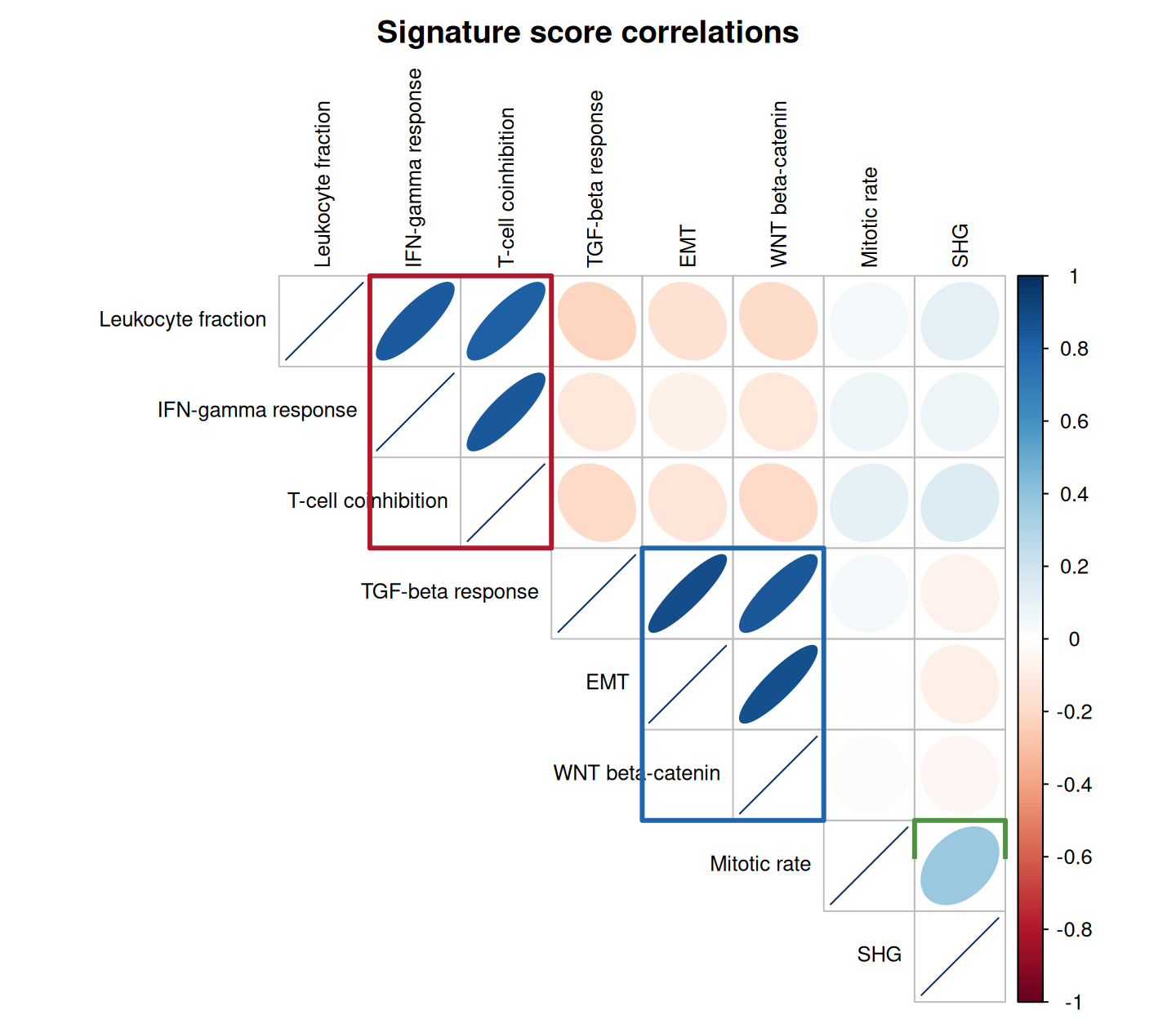
The three rectangles group the signatures into co-varying modules — the structure the reference paper boxed around its consensus clusters.
2. Clustering Samples into Immune Subtypes
## The reference uses ConsensusClusterPlus; hierarchical clustering on the
## z-scored matrix is the dependency-free stand-in
z_mat <- t(scale(sig_mat))     # signatures x samples, each signature z-scored
hcs <- hclust(dist(t(z_mat)), method = "ward.D2")
n_sub <- 6
subtype <- paste0("C", cutree(hcs, k = n_sub))

col_fun <- circlize::colorRamp2(c(-2, 0, 2), c("#2166AC", "white", "#B2182B"))
ha <- HeatmapAnnotation(Subtype = subtype,
                        col = list(Subtype = c("C1" = "#F2CCCC", "C2" = "#B31E22",
                                               "C3" = "#529B40", "C4" = "#020105",
                                               "C5" = "#383D8E", "C6" = "#EABF00")),
                        show_legend = FALSE)
Heatmap(z_mat, name = "Score (z)", top_annotation = ha,
        col = col_fun, cluster_columns = hcs,
        show_column_names = FALSE,
        row_names_gp = grid::gpar(fontsize = 8),
        column_split = 6,          # with a dendrogram, split takes k, not a factor
        column_gap = unit(1.5, "mm"),
        border = TRUE)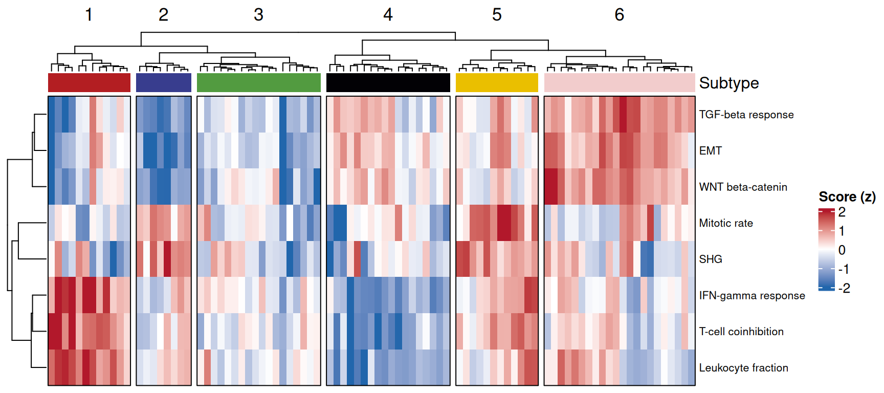
Each column split is one subtype; the colour blocks show which signatures dominate it. With real data the assignment step is the author’s ImmuneSubtypeClassifier package, which is more robust than the original pipeline.
3. Score Distributions per Subtype
show_sigs <- c("Leukocyte fraction", "TGF-beta response", "Mitotic rate")
dist_df <- sig_scores |>
  mutate(subtype = subtype) |>
  pivot_longer(all_of(show_sigs), names_to = "Signature", values_to = "Score")

ggplot(dist_df, aes(subtype, Score, fill = subtype)) +
  geom_boxplot(outlier.shape = NA, width = 0.65) +
  geom_hline(yintercept = 0, linetype = "dashed", colour = "grey40") +
  facet_wrap(~Signature, nrow = 1) +
  scale_fill_manual(values = c("C1" = "#F2CCCC", "C2" = "#B31E22", "C3" = "#529B40",
                               "C4" = "#020105", "C5" = "#383D8E", "C6" = "#EABF00")) +
  labs(x = NULL, y = "Signature score", fill = "Subtype") +
  theme_classic(base_size = 11) +
  theme(legend.position = "top", legend.key.size = unit(3, "mm"))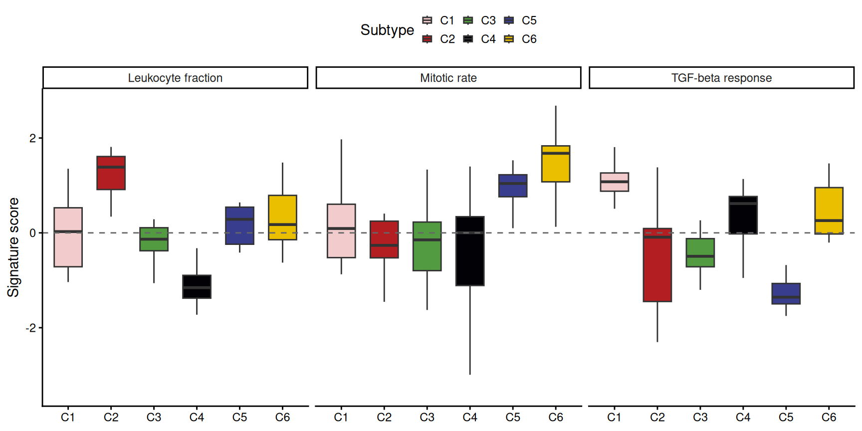
Tip
Practice tips
- The reference pipeline is sensitive to the gene-quantification method — it does not work well on FPKM/RPKM/TPM; use the author’s
ImmuneSubtypeClassifierfor real data. - Subtypes are named by their dominant modules (e.g. C2 = IFN-γ dominant, C6 = TGF-β dominant); with simulated data the box panels let you assign such names by eye.
- Keep the module heatmap and the subtype split in one figure: reviewers check that the modules used for clustering are the ones the subtypes differ on.
Application
Immune-subtype assignment is the standard first annotation in immuno-oncology cohorts: it groups tumours before checkpoint-response or TMB comparisons. The layout above (module heatmap → subtype strip → score distributions) mirrors how the reference figure reports them.
Reference
[1] Thorsson V, Gibbs DL, Brown SD, et al. The immune landscape of cancer. Immunity. 2018;48(4):812-830.e24. doi:10.1016/j.immuni.2018.03.023
[2] Xiaofan Lu, et al. FigureYa: A Standardized Visualization Framework for Enhancing Biomedical Data Interpretation and Research Efficiency. iMetaMed. 2025. doi:10.1002/imm3.70005