Pie Matrix

Note

Hiplot website

This page is the tutorial for source code version of the Hiplot Pie Matrix plugin. You can also use the Hiplot website to achieve no code ploting. For more information please see the following link:

https://hiplot.cn/basic/pie-matrix?lang=en

Setup

• System Requirements: Cross-platform (Linux/MacOS/Windows)

• Programming language: R

• Dependent packages: data.table; jsonlite; ggplot2; dplyr; tidyr; stringr

# Install packages
if (!requireNamespace("data.table", quietly = TRUE)) {
  install.packages("data.table")
}
if (!requireNamespace("jsonlite", quietly = TRUE)) {
  install.packages("jsonlite")
}
if (!requireNamespace("ggplot2", quietly = TRUE)) {
  install.packages("ggplot2")
}
if (!requireNamespace("dplyr", quietly = TRUE)) {
  install.packages("dplyr")
}
if (!requireNamespace("tidyr", quietly = TRUE)) {
  install.packages("tidyr")
}
if (!requireNamespace("stringr", quietly = TRUE)) {
  install.packages("stringr")
}

# Load packages
library(data.table)
library(jsonlite)
library(ggplot2)
library(dplyr)
library(tidyr)
library(stringr)

sessioninfo::session_info("attached")

─ Session info ───────────────────────────────────────────────────────────────
 setting  value
 version  R version 4.5.2 (2025-10-31)
 os       Ubuntu 24.04.3 LTS
 system   x86_64, linux-gnu
 ui       X11
 language (EN)
 collate  C.UTF-8
 ctype    C.UTF-8
 tz       UTC
 date     2026-01-17
 pandoc   3.1.3 @ /usr/bin/ (via rmarkdown)
 quarto   1.8.27 @ /usr/local/bin/quarto

─ Packages ───────────────────────────────────────────────────────────────────
 package    * version date (UTC) lib source
 data.table * 1.18.0  2025-12-24 [1] RSPM
 dplyr      * 1.1.4   2023-11-17 [1] RSPM
 ggplot2    * 4.0.1   2025-11-14 [1] RSPM
 jsonlite   * 2.0.0   2025-03-27 [1] RSPM
 stringr    * 1.6.0   2025-11-04 [1] RSPM
 tidyr      * 1.3.2   2025-12-19 [1] RSPM

 [1] /home/runner/work/_temp/Library
 [2] /opt/R/4.5.2/lib/R/site-library
 [3] /opt/R/4.5.2/lib/R/library
 * ── Packages attached to the search path.

──────────────────────────────────────────────────────────────────────────────

Data Preparation

# Load data
data <- data.table::fread(jsonlite::read_json("https://hiplot.cn/ui/basic/pie-matrix/data.json")$exampleData$textarea[[1]])
data <- as.data.frame(data)

# Convert data structure
data[,"genre"] <- factor(data[,"genre"], levels = unique(data[,"genre"]))
data[,"mpaa"] <- factor(data[,"mpaa"], levels = unique(data[,"mpaa"]))
data[,"status"] <- factor(data[,"status"], levels = unique(data[,"status"]))
col <- c("#E64B35FF","#4DBBD5FF")
df <- matrix(NA, nrow = length(unique(data[,"mpaa"])),
             ncol = length(unique(data[,"genre"])))
row.names(df) <- unique(data[,"mpaa"])
colnames(df) <- unique(data[,"genre"])
for (i in 1:nrow(df)) {
    for (j in 1:ncol(df)) {
      for (k in unique(data[,"status"])) {
        if (is.na(df[i, j])) {
          df[i, j] <- sum(data[,"genre"] == unique(data[,"genre"])[j] &
            data[,"mpaa"] == unique(data[,"mpaa"])[i] &
            data[,"status"] == k)
        } else {
          df[i, j] <- paste0(df[i, j], ",", 
            sum(data[,"genre"] == unique(data[,"genre"])[j] &
              data[,"mpaa"] == unique(data[,"mpaa"])[i] &
              data[,"status"] == k))
        }
      }
    }
}
df <- as.matrix(df)

# View data
head(data[,1:5])

                                               title year length budget rating
1                          Shawshank Redemption, The 1994    142     25    9.1
2     Lord of the Rings: The Return of the King, The 2003    251     94    9.0
3 Lord of the Rings: The Fellowship of the Ring, The 2001    208     93    8.8
4             Lord of the Rings: The Two Towers, The 2002    223     94    8.8
5                                       Pulp Fiction 1994    168      8    8.8
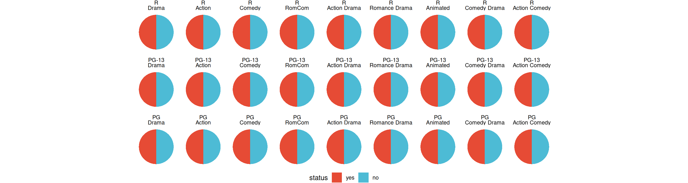
6                                   Schindler's List 1993    195     25    8.8

Visualization

# Pie Matrix
p <- df %>% as.table() %>%
  as.data.frame() %>%
  mutate(Freq = str_split(Freq,",")) %>%
  unnest(Freq) %>%
  mutate(Freq = as.integer(Freq)) %>%
  # Convert the values to a percentage (which adds up to 1 for each graph)
  group_by(Var1, Var2) %>%
  mutate(Freq = ifelse(is.na(Freq), NA, Freq / sum(Freq)),
         color = row_number()) %>%
  ungroup() %>%
  # Plot
  ggplot(aes("", Freq, fill=factor(color, labels = unique(data[,"status"])))) + 
  geom_bar(width = 2, stat = "identity") +
  coord_polar("y") +
  facet_wrap(~Var1+Var2, ncol = ncol(df)) +
  scale_fill_manual(values = col) +
  theme_void() +
  theme(axis.text = element_blank(), axis.ticks = element_blank(),
        panel.grid = element_blank(), axis.title = element_blank(),
        legend.position = "bottom", legend.direction = "horizontal") +
  guides(fill = guide_legend(nrow = 1, title = "status"))
  
p

Figure 1: Pie Matrix