# Installing packages
if (!requireNamespace("syntR", quietly = TRUE)) {
  remotes::install_github("ksamuk/syntR")
}

# Load packages
library(syntR)Synteny Blocks Plot
Collinearity is widely used in the study of complex genomes. This tutorial, based on the R package syntR, summarizes the identification of shared collinearity blocks between two genetic maps, chromosomal rearrangements, and their mapping.
Example
Setup
System Requirements: Cross-platform (Linux/MacOS/Windows)
Programming language: R
Dependent packages:
syntR
sessioninfo::session_info("attached")─ Session info ───────────────────────────────────────────────────────────────
setting value
version R version 4.6.0 (2026-04-24)
os Ubuntu 24.04.4 LTS
system x86_64, linux-gnu
ui X11
language (EN)
collate C.UTF-8
ctype C.UTF-8
tz UTC
date 2026-05-09
pandoc 3.1.3 @ /usr/bin/ (via rmarkdown)
quarto 1.9.37 @ /usr/local/bin/quarto
─ Packages ───────────────────────────────────────────────────────────────────
package * version date (UTC) lib source
dplyr * 1.2.1 2026-04-03 [1] RSPM
intervals * 0.15.5 2024-08-23 [1] RSPM
magrittr * 2.0.5 2026-04-04 [1] RSPM
reshape2 * 1.4.5 2025-11-12 [1] RSPM
syntR * 1.0 2026-05-04 [1] Github (ksamuk/syntR@bce120c)
tidyr * 1.3.2 2025-12-19 [1] RSPM
viridis * 0.6.5 2024-01-29 [1] RSPM
viridisLite * 0.4.3 2026-02-04 [1] RSPM
[1] /home/runner/work/_temp/Library
[2] /opt/R/4.6.0/lib/R/site-library
[3] /opt/R/4.6.0/lib/R/library
* ── Packages attached to the search path.
──────────────────────────────────────────────────────────────────────────────Data Preparation
syntR requires marker positions from two genetic maps (chromosome and map position for each marker). Before using syntR, the marker order must be inferred for each map. Before using syntR for mapping, positional data for individual markers (e.g., SNPs, microsatellites, etc.) from the two maps can be obtained using R/qtl, ASMap, and Lep-MAP. Alternatively, the alignment results can be converted to similar input files for analysis and mapping using minimap2.
# load the example marker data
data(ann_pet_map)
head(ann_pet_map)
map1_name map1_chr map1_pos map2_name map2_chr map2_pos
1 HanXRQChr12_10463750 Ann12 23.33200 HanXRQChr12_10463750 Pet12_16 0.000000
2 HanXRQChr12_10463069 Ann12 23.33091 HanXRQChr12_10463069 Pet12_16 3.660274
3 HanXRQChr12_67274477 Ann12 51.14234 HanXRQChr12_67274477 Pet12_16 3.660274
4 HanXRQChr12_11545866 Ann12 25.01880 HanXRQChr12_11545866 Pet12_16 3.660274
5 HanXRQChr12_11545707 Ann12 25.01856 HanXRQChr12_11545707 Pet12_16 3.660274
6 HanXRQChr12_9937279 Ann12 22.47337 HanXRQChr12_9937279 Pet12_16 4.567248The data is organized into six columns:
-
map1_name: A unique identifier for the marker. In this example, the marker is named based on its position in the reference genome (determined by aligning GBS reads). -
map1_chr: The chromosome number of the marker in the first map. -
map1_pos: The position of the marker in the first map (e.g., in centimeters). -
map2_name: Same as above, but for map 2. These names may or may not be the same asmap1_names. -
map2_chr: The chromosome number of the marker in the second map. -
map2_pos: The position of the marker in the second map.
The example data is generated by comparing GBS data of two butterflies, Helianthus petiolaris ssp. petiolaris and H. petiolaris ssp. fallax. First, load the marker data (ann_pet_map) and the chromosome length list of map1 (ann_chr_lengths), and convert it into a list with three elements (marker data, the position of the chromosome break between map1 and map2) through the make_one_map function:
# read in list of chromosome lengths for map1
# this is an optional file that defines the maximum
# length of each chromosome (in cM) if this is known
# NB: this is useful when the markers being compared
# do not cover the entire map
data(ann_chr_lengths)
ann_chr_lengths
map1_chr map1_max_chr_lengths
1 Ann08 63.68
2 Ann09 96.46
3 Ann12 71.68
4 Ann15 80.29
5 Ann16 103.49
6 Ann17 97.14# make_one_map places all the markers on a single scale
# and adds padding between the chromosomes
# to aid the algorithm and for visualization purposes
map_list <- make_one_map(ann_pet_map, map1_max_chr_lengths = ann_chr_lengths)Visualization
1. Adjust the order of the graphs
Use plot_maps() to create a basic bitmap of labeled data:
# Adjust the order of the graphs
plot_maps(map_df = map_list[[1]], map1_chrom_breaks = map_list[[2]], map2_chrom_breaks = map_list[[3]])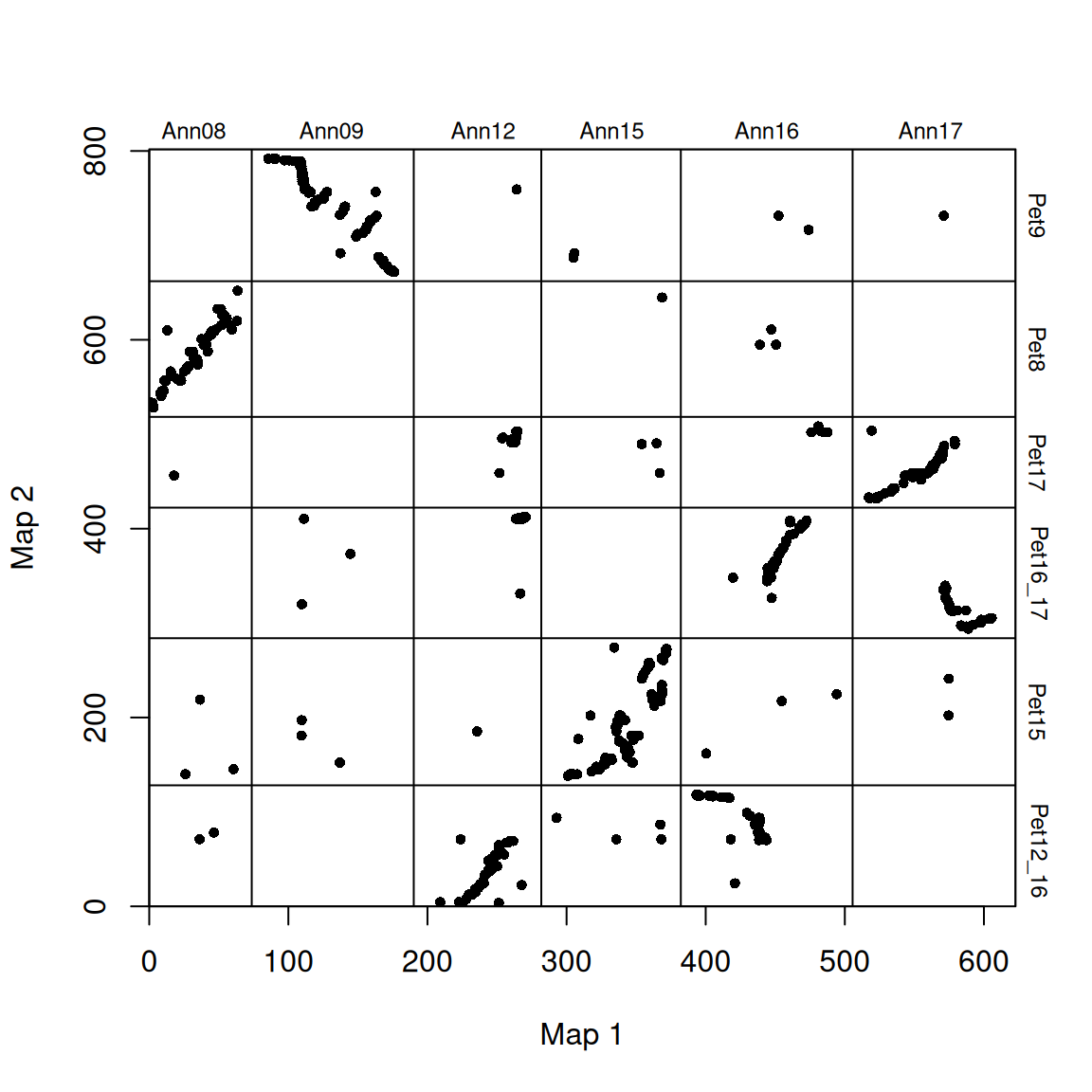
Chromosomes are labeled with species-specific names, and chromosome breaks are indicated by horizontal and vertical lines.
Because the chromosomes are ordered arbitrarily (chromosomes have no inherent order), these diagrams appear quite scattered. To improve readability, the order of the chromosomes of species 2 can be rearranged to align with that of species 1 (plotted along the x-axis). Any “completely upside-down” chromosomes can also be rotated so that they align along a 1:1 line (in terms of chromosomal proportions).
# Adjust the order of the graphs
map2_chr_order <- c("Pet8", "Pet9", "Pet12_16", "Pet15", "Pet16_17", "Pet17")
flip_chrs <- c("Pet9")
map_list <- make_one_map(ann_pet_map, map1_max_chr_lengths = ann_chr_lengths, map2_chr_order = map2_chr_order, flip_chrs = flip_chrs)
plot_maps(map_df = map_list[[1]], map1_chrom_breaks = map_list[[2]], map2_chrom_breaks = map_list[[3]])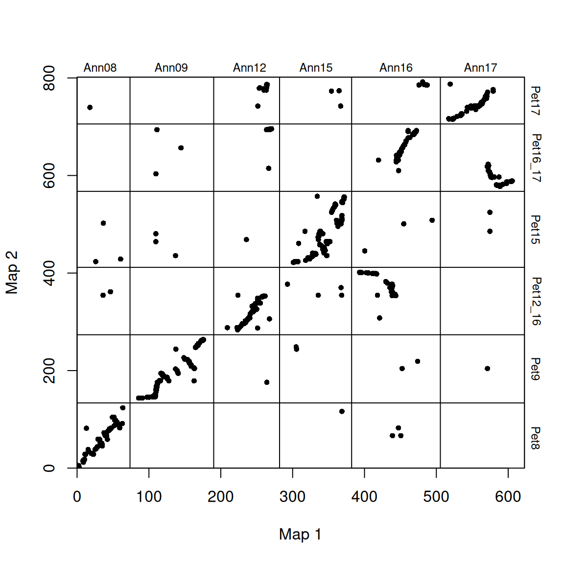
2. Determining the optimal flipping parameters
The key tuning parameters for the syntR algorithm are max_cluster_range (CR max), followed by max_nn_dist (NN dist). max_cluster_range determines the maximum size of marker clusters that will be collapsed into a single point for further analysis. It defines the maximum distance that clustered markers can span. Larger values for max_cluster_range result in more markers clustered into a single point.
max_nn_dist determines which markers are considered outliers and removed from further analysis. Markers with no adjacent markers within the max_nn_dist range are considered outliers. Larger values for max_nn_dist result in fewer markers being removed.
A simple way to find the optimal combination of these two parameters is to fit a range of values for both parameters and choose the value that maximizes the coverage (the percentage of the map assigned to the same block) of both maps and minimizes the number of outliers (“Combined” in the figure below is the sum of the ratios of these metrics).
The method for selecting the best CR max and NN dist is: (1) run syntR with a range of parameter combinations; (2) save summary statistics about the genetic distance for each map represented in the homology block and the number of markers retained for each run; (3) find the parameter combination that maximizes the average weighted composite statistic of these three measures. In the case of multiple local maxima, the local maximum with the smallest CR max value is selected to reduce the number of potential false positives.
This step can be skipped by using the default values of max_cluster_range = 2 and max_nn_dist = 10. This parameter is likely to be well suited for most genetic maps.
# find best parameter combination
# run find_synteny_blocks with each parameter combination and collect summary statistics

parameter_data <- test_parameters(map_list, max_cluster_range_list = seq(1, 5, by = 0.5), max_nn_dist_list = seq(10, 50, by = 10))
plot_summary_stats(parameter_data[[1]], "composite")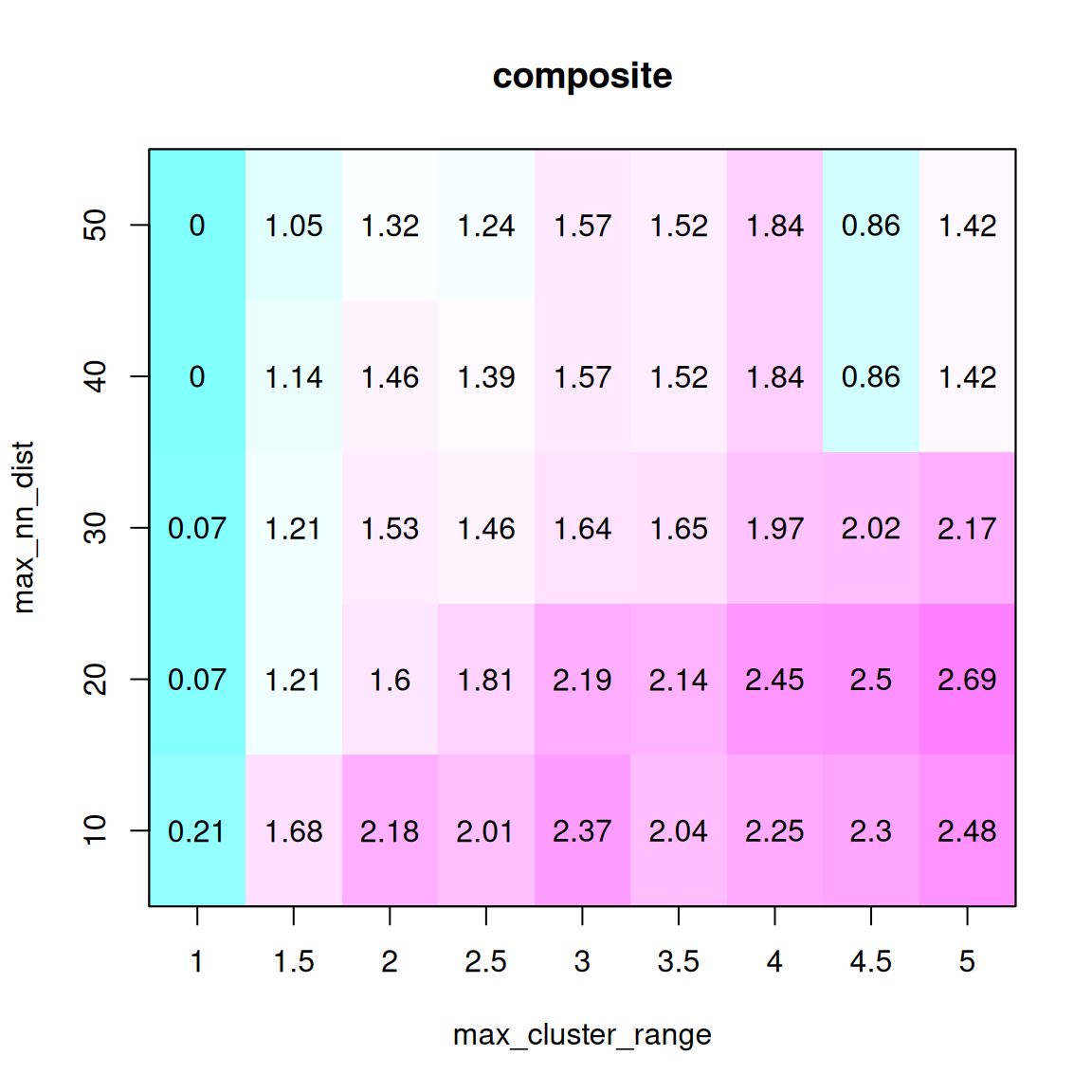
In this example, choose max_cluster_range to be 2 and max_nn_dsit to be 10.
3. Find synteny blocks
After determining the two tuning parameters, we can run the main syntR function: find_synteny_blocks. This function takes a set of labeled data (contained in the map_list object we created earlier) and runs it through the algorithm described by Ostevik et al. to perform error detection and homology block identification. To run it:
# Find synteny blocks
synt_blocks <- find_synteny_blocks(map_list, max_cluster_range = 2, max_nn_dist = 10, plots = TRUE)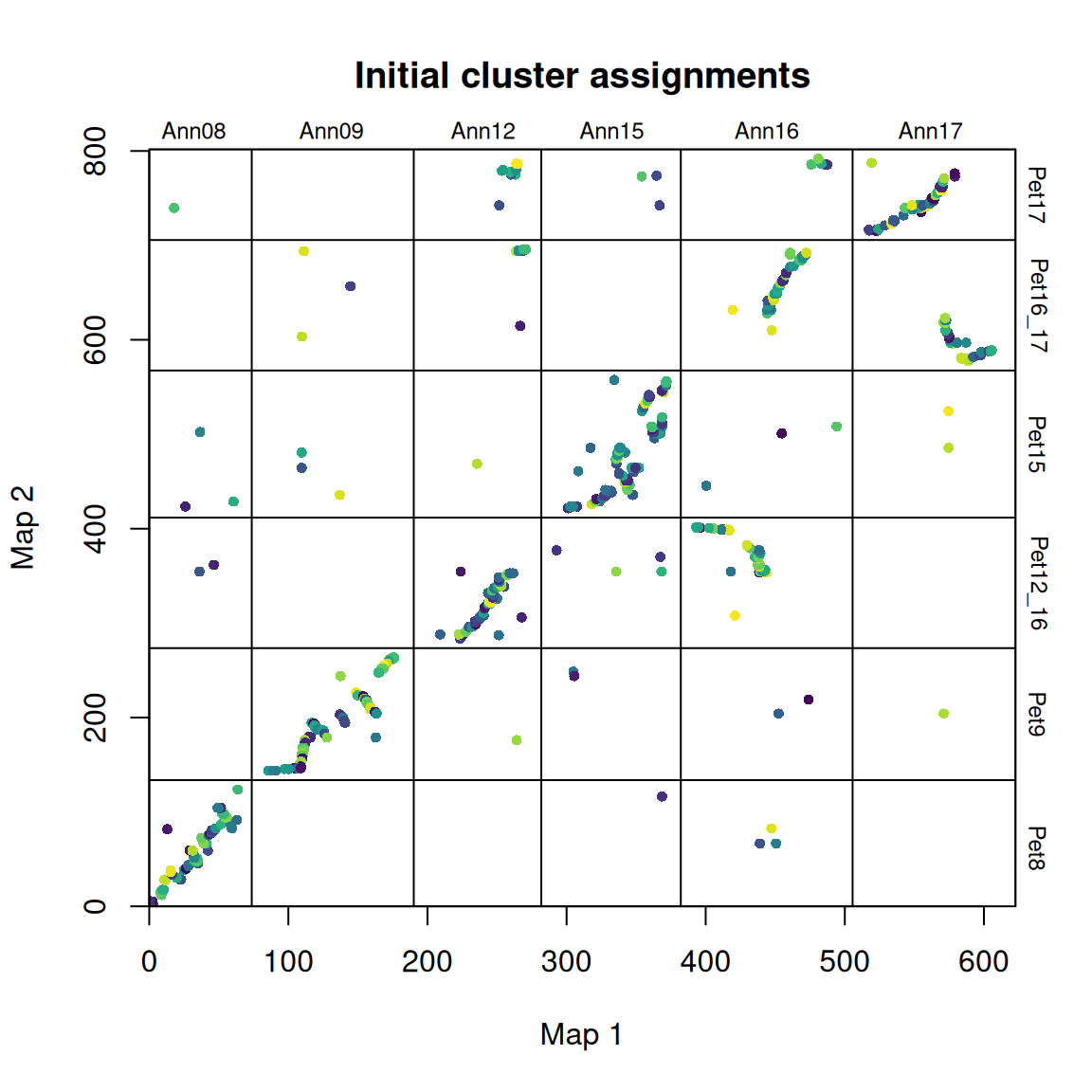
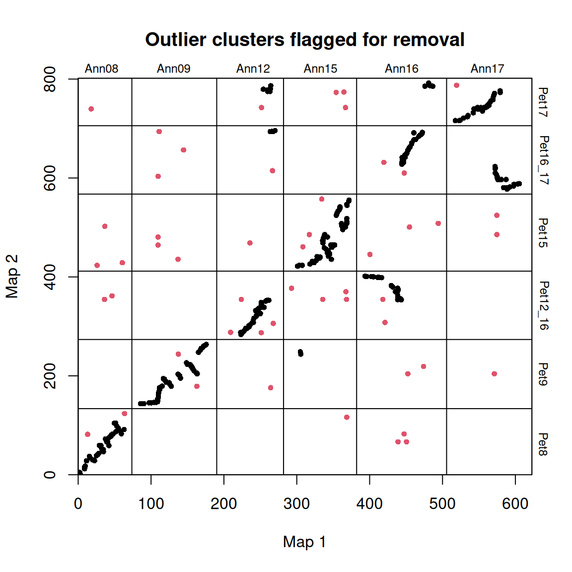
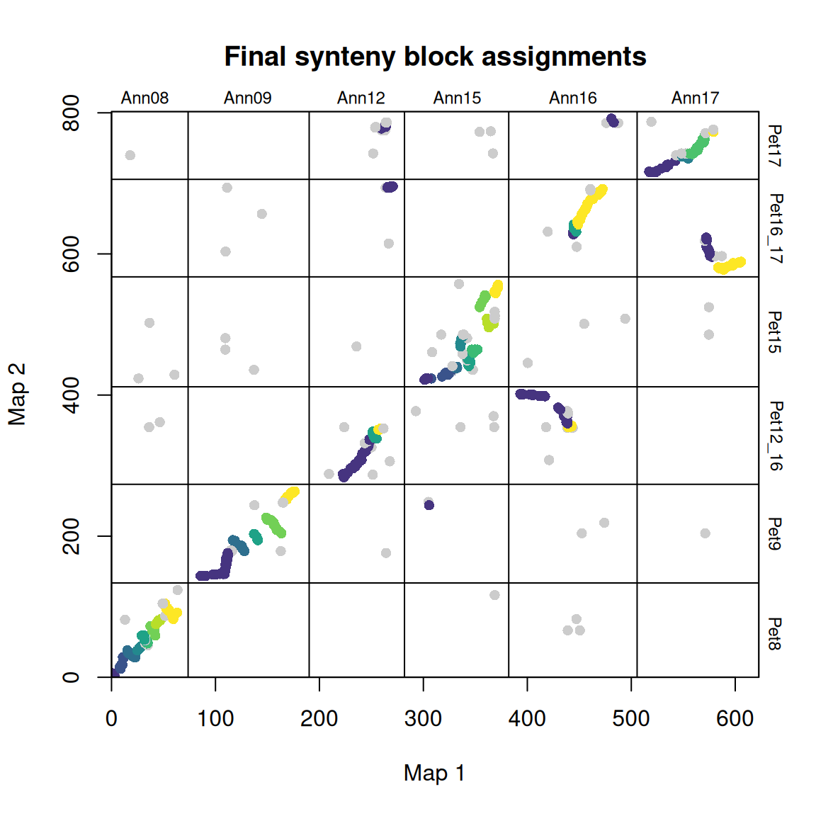
When plots=TRUE is specified, the function generates three plots showing the algorithm’s progress. In the first plot, the mapping errors are smoothed using a pre-clustering step. Next, outliers are labeled and removed. Finally, homologous blocks are identified using the syntR Friends clustering algorithm.
find_synteny_blocks outputs a list object containing five data frames:
# print the contents of synt_blocks

lapply(synt_blocks, head)
$marker_df
map1_name map1_chr map1_pos map1_posfull map2_name
1 HanXRQChr12_10463750 Ann12 23.33200 223.4720 HanXRQChr12_10463750
2 HanXRQChr12_10463069 Ann12 23.33091 223.4709 HanXRQChr12_10463069
3 HanXRQChr12_67274477 Ann12 51.14234 251.2823 HanXRQChr12_67274477
4 HanXRQChr12_11545866 Ann12 25.01880 225.1588 HanXRQChr12_11545866
5 HanXRQChr12_11545707 Ann12 25.01856 225.1586 HanXRQChr12_11545707
6 HanXRQChr12_9937279 Ann12 22.47337 222.6134 HanXRQChr12_9937279
map2_chr map2_pos map2_posfull cluster block final_block orientation
1 Pet12_16 0.000000 283.4780 1 2 2 positive
2 Pet12_16 3.660274 287.1382 2 2 2 positive
3 Pet12_16 3.660274 287.1382 3 <NA> NA outlier
4 Pet12_16 3.660274 287.1382 4 2 2 positive
5 Pet12_16 3.660274 287.1382 4 2 2 positive
6 Pet12_16 4.567248 288.0452 2 2 2 positive
$synteny_blocks_df
block map1_chr map1_start map1_end map2_chr map2_start map2_end
1 5 Ann08 0.307917 3.096819 Pet8 0.00000 5.872578
2 6 Ann08 7.970652 11.630196 Pet8 12.06862 28.437648
3 7 Ann08 15.356354 22.979486 Pet8 28.43765 38.207576
4 8 Ann08 24.903278 28.616233 Pet8 38.20758 43.602465
5 9 Ann08 32.578270 34.839079 Pet8 48.02882 50.686116
6 10 Ann08 29.056599 32.577711 Pet8 51.58404 59.123579
orientation
1 negative
2 positive
3 negative
4 positive
5 unclassified
6 negative
$map1_breaks
start end
1 3.096819 7.970652
2 11.630196 15.356354
3 22.979486 24.903278
4 28.616233 29.056599
5 32.577711 32.578270
6 34.839079 37.529721
$map2_breaks
start end
1 5.872578 12.06862
2 28.437648 28.43765
3 38.207576 38.20758
4 43.602465 48.02882
5 50.686116 51.58404
6 59.123579 59.12358
$summary_stats
num_blocks map1_coverage map2_coverage n_outliers
1 41 382.8091 567.0453 205These elements are:
$marker_df, a data frame containing the original list of markers and their homologous block assignments.$synteny_blocks_df, a data frame summarizing the span of each homologous block in each map (in map units), and the inferred orientation (juxtaposed, inverted, etc.) of homologous blocks with sufficient evidence for orientation.$map1_breaks, a data frame listing the breakpoints between synthetic blocks in map1.$map2_breaks, a data frame listing the breakpoints between synthetic blocks in map2.$summary_stats, a data frame summarizing the algorithm results (coverage, etc.)
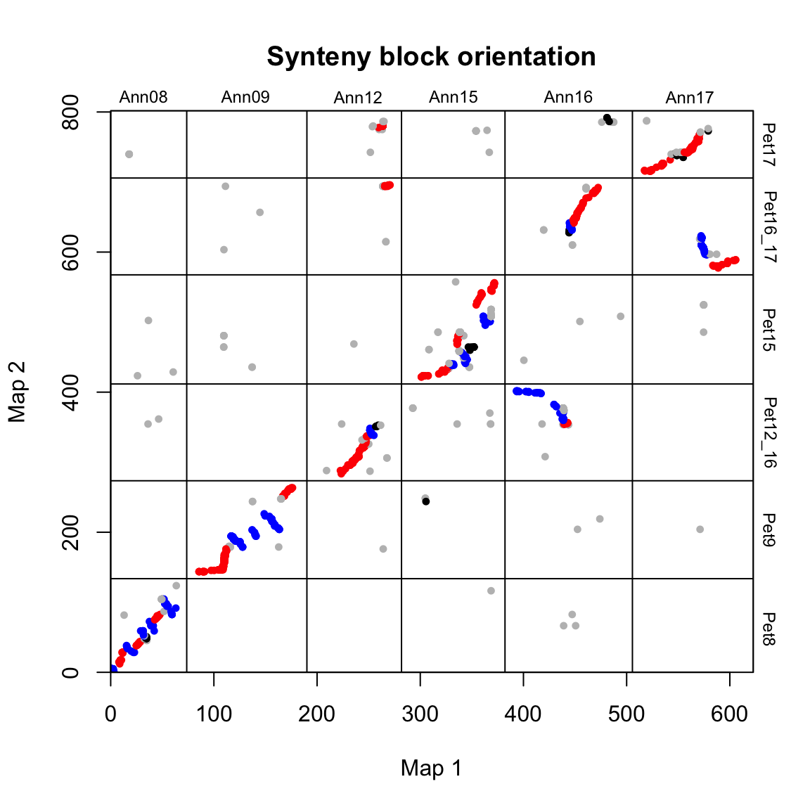
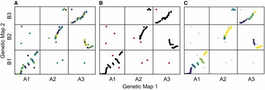
The orientation of the blocks can be plotted as shown below:
# Plot synteny block orientations
synt_blocks[[1]] %>%
    plot_maps(map_list[[2]], map_list[[3]], col = c("blue", "grey", "red", "black")[as.numeric(as.factor(.$orientation))],
              main = "Synteny block orientation",  cex_val = 0.75)
In this case, blue = inverted, red = syntenic, and grey/black = unclassified.
Application
Reference
[1] Ostevik, Kate L., Kieran Samuk, and Loren H. Rieseberg. “Ancestral reconstruction of karyotypes reveals an exceptional rate of nonrandom chromosomal evolution in sunflower.” Genetics 214, no. 4 (2020): 1031-1045.