# Installing necessary packages
if (!requireNamespace("tidycmprsk", quietly = TRUE)) {
  install.packages("tidycmprsk")
}
if (!requireNamespace("ggsurvfit", quietly = TRUE)) {
  install.packages("ggsurvfit")
}

# Load packages
library(survival)
library(tidycmprsk)
library(ggsurvfit)
library(ggplot2)
library(dplyr)Competing Risk Cumulative Incidence
When patients can fail from more than one cause — progression or death, relapse or transplant mortality — standard Kaplan–Meier analysis is wrong for the event of interest: censoring patients at their competing event pretends they were still at risk of progressing, and the naive 1 − KM estimator overestimates the incidence, dramatically so when the competing event is common [1]. The correct descriptive tool is the cumulative incidence function (CIF, Aalen–Johansen estimator), which treats competing events as competing: a subject who dies can no longer progress, and the CIFs of all causes sum to 1.
Group comparison uses Gray’s test (a K-sample test on the CIFs), and regression uses the Fine–Gray subdistribution hazard model [2]. This tutorial walks through all three with tidycmprsk [3] and ggsurvfit [4], on the classic mgus2 cohort [5]: 1,384 patients with monoclonal gammopathy of undetermined significance, where progression to plasma cell malignancy competes with death.
This tutorial covers four workflows:
- CIFs of both competing outcomes with confidence intervals and risk table;
- CIFs by a covariate with Gray’s test;
- Fine–Gray subdistribution hazard regression;
- Why 1 − KM overestimates incidence — the comparison every reviewer asks for.
Example
Setup
System Requirements: Cross-platform (Linux/MacOS/Windows)
Programming language: R
Dependent packages:
survival;tidycmprsk;ggsurvfit;ggplot2;dplyr
sessioninfo::session_info("attached")─ Session info ───────────────────────────────────────────────────────────────
setting value
version R version 4.6.2 (2026-10-29)
os Ubuntu 24.04.5 LTS
system x86_64, linux-gnu
ui X11
language (EN)
collate C.UTF-8
ctype C.UTF-8
tz UTC
date 2026-10-31
pandoc 3.1.3 @ /usr/bin/ (via rmarkdown)
quarto 1.10.20 @ /usr/local/bin/quarto
─ Packages ───────────────────────────────────────────────────────────────────
! package * version date (UTC) lib source
P dplyr * 1.2.1 2026-04-03 [?] RSPM
P ggplot2 * 4.0.3.9000 2026-10-30 [?] Github (tidyverse/ggplot2@b638d65)
ggsurvfit * 1.2.1 2026-07-24 [1] RSPM
P survival * 3.8-6 2026-01-16 [?] RSPM
tidycmprsk * 1.1.2 2026-04-09 [1] RSPM
[1] /home/runner/.cache/R/renv/library/Bizard-5140bdc6/linux-ubuntu-noble/R-4.6/x86_64-pc-linux-gnu
[2] /home/runner/work/_temp/Library
[3] /opt/R/4.6.2/lib/R/library
* ── Packages attached to the search path.
P ── Loaded and on-disk path mismatch.
──────────────────────────────────────────────────────────────────────────────Data Preparation
mgus2 ships with the survival package [5]: 1,384 MGUS patients followed from diagnosis for progression to a plasma cell malignancy (PCM) or death. Follow-up time is the earlier of progression (ptime) and last contact (futime); the competing-risks event code is 0 = censored, 1 = PCM (the event of interest), 2 = death (the competing event).
data(mgus2)

mgus2$etime <- with(mgus2, ifelse(pstat == 1, ptime, futime))
mgus2$event <- with(mgus2, ifelse(pstat == 1, 1, ifelse(death == 1, 2, 0)))
mgus2$event_f <- factor(mgus2$event, levels = 0:2,
                        labels = c("censored", "pcm", "death"))

cat("Patients:", nrow(mgus2),
    "| progression:", sum(mgus2$event == 1),
    "| death (competing):", sum(mgus2$event == 2), "\n")
Patients: 1384 | progression: 115 | death (competing): 860 Visualization
1. Cumulative Incidence of Both Outcomes
ci1 <- cuminc(Surv(etime, event_f) ~ 1, data = mgus2)

ggcuminc(ci1, outcome = c("pcm", "death")) +
  add_confidence_interval() +
  add_risktable(size = 3) +
  scale_color_manual(values = c(pcm = "#B2182B", death = "#2166AC"), name = NULL) +
  scale_fill_manual(values = c(pcm = "#B2182B", death = "#2166AC"), guide = "none") +
  xlab("Months since diagnosis") +
  ylab("Cumulative incidence") +
  theme_bw(base_size = 11)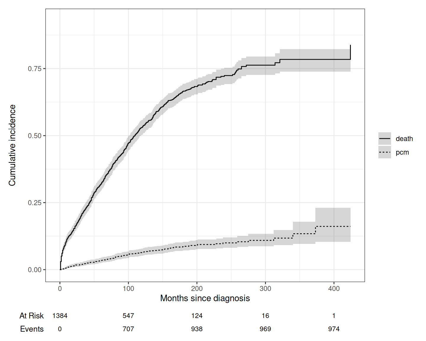
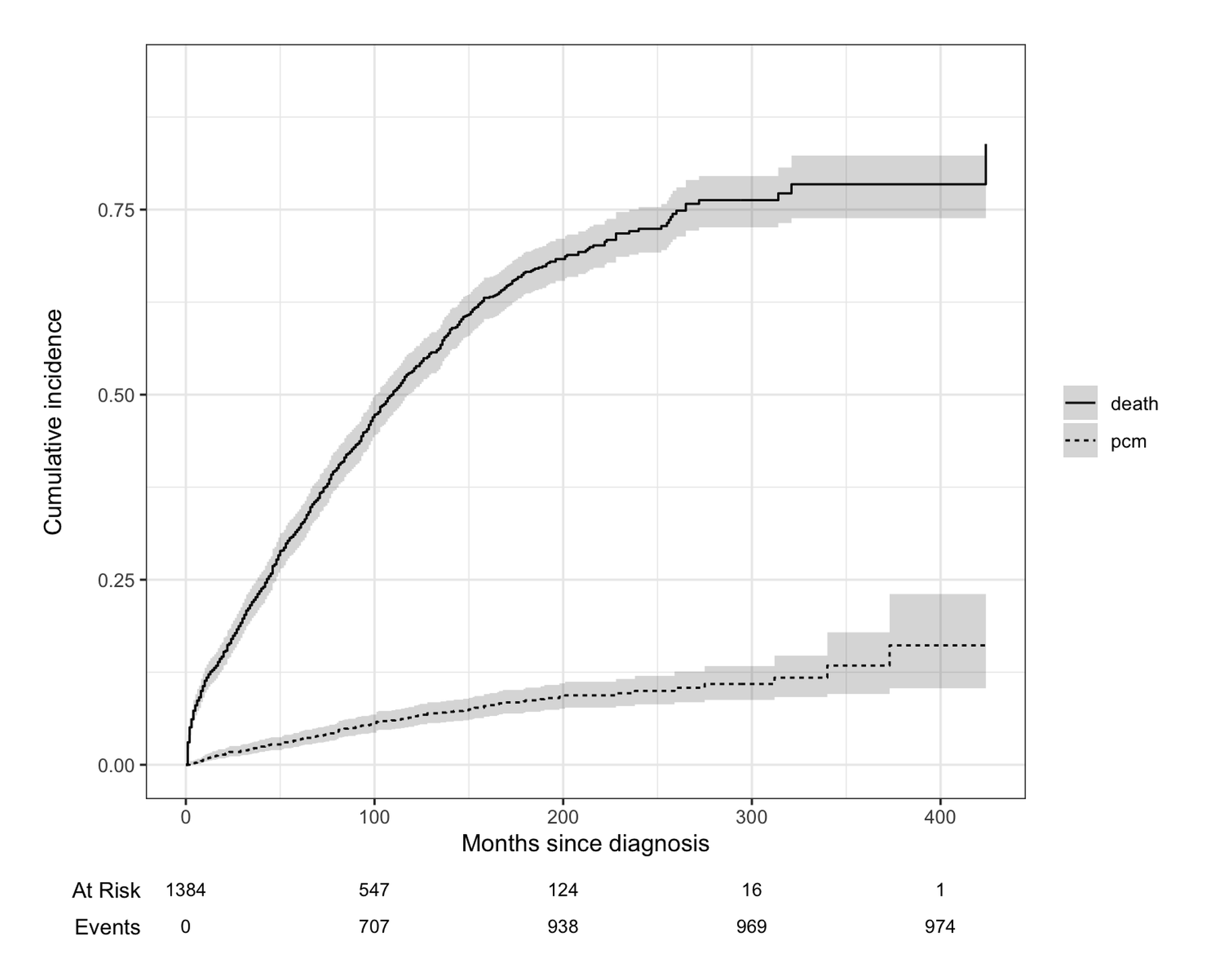
Death dominates: by 20 years roughly 78% have died versus about 16% who have progressed — which is exactly the setting where naive Kaplan–Meier analysis of progression goes wrong (Section 4).
2. Comparing Groups with Gray’s Test
ci2 <- cuminc(Surv(etime, event_f) ~ sex, data = mgus2)
gt <- glance(ci2)
cat(sprintf("Gray's test, progression: chi-square = %.2f, df = %d, p = %.3f\n",
            gt$statistic_1, gt$df_1, gt$p.value_1))
Gray's test, progression: chi-square = 1.19, df = 1, p = 0.274cat(sprintf("Gray's test, death: chi-square = %.2f, df = %d, p = %.3f\n",
gt$statistic_2, gt$df_2, gt$p.value_2))Gray's test, death: chi-square = 11.65, df = 1, p = 0.001ggcuminc(ci2, outcome = "pcm") +
add_confidence_interval() +
scale_color_manual(values = c(F = "#1B9E77", M = "#7570B3"), name = "Sex") +
scale_fill_manual(values = c(F = "#1B9E77", M = "#7570B3"), guide = "none") +
xlab("Months since diagnosis") +
ylab("Cumulative incidence of progression") +
theme_bw(base_size = 11)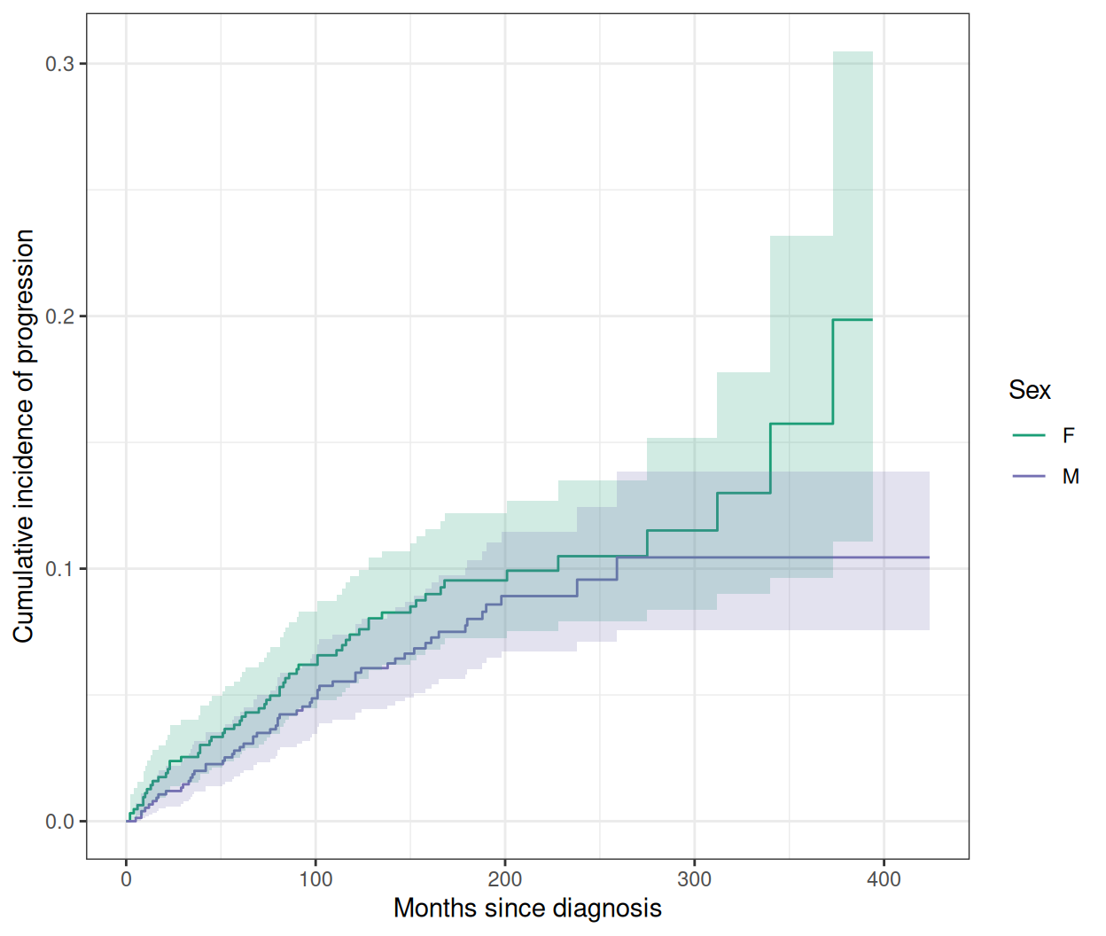
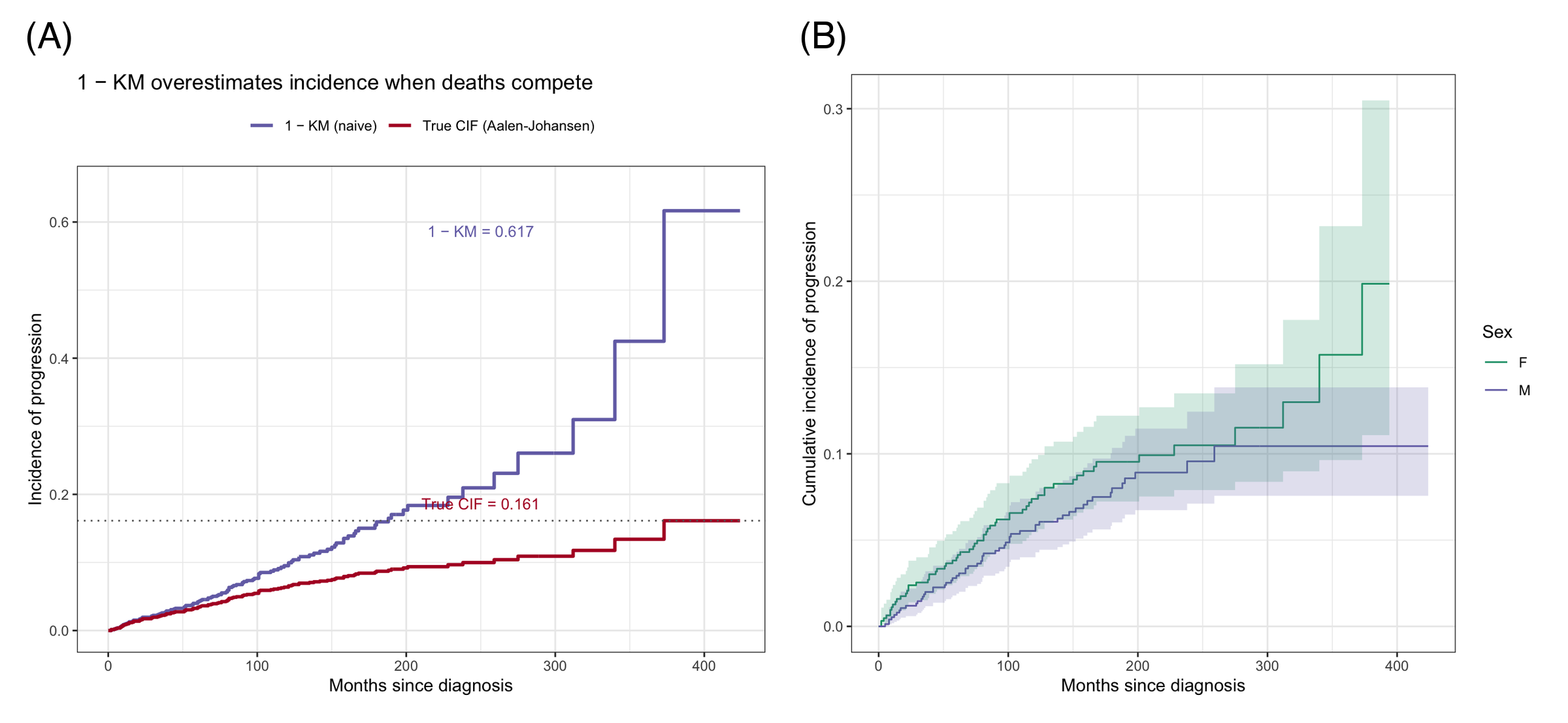
Men progress slightly faster than women, but Gray’s test does not reach significance at the 0.05 level — with the effect quantified properly by the regression below.
3. Fine-Gray Regression
fg <- crr(Surv(etime, event_f) ~ sex + age, data = mgus2, failcode = "pcm")
fgdf <- tidy(fg, exponentiate = TRUE, conf.int = TRUE) |>
  mutate(term_lbl = recode(term, sexM = "Sex: M vs F", age = "Age (per year)"))

ggplot(fgdf, aes(x = estimate, y = term_lbl)) +
  geom_errorbar(aes(xmin = conf.low, xmax = conf.high), orientation = "y",
                width = 0.12, color = "#B2182B") +
  geom_point(size = 3, color = "#B2182B") +
  geom_vline(xintercept = 1, linetype = "dashed", color = "grey40") +
  scale_x_log10() +
  labs(x = "Subdistribution hazard ratio (log scale)", y = NULL,
       title = "Fine-Gray regression: progression to malignancy") +
  theme_bw(base_size = 11)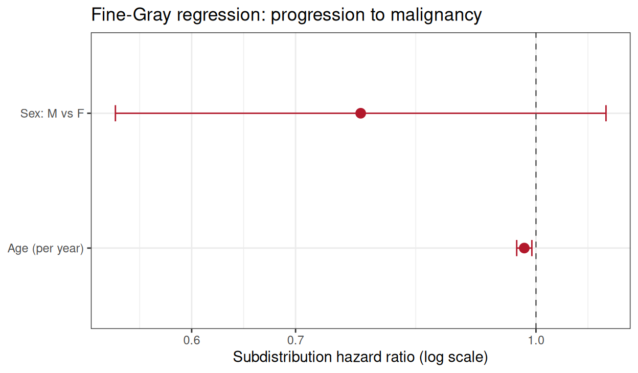
The subdistribution HR answers the clinically relevant question — how the covariate shifts the absolute incidence of progression in the presence of the competing risk. For the etiologic (cause-specific) question, fit survival::coxph instead and say which one you report.
4. Why 1 − KM Overestimates: The Comparison Figure
kmfit <- survfit(Surv(etime, event == 1) ~ 1, data = mgus2)  # deaths censored
kmdf <- data.frame(time = kmfit$time, est = 1 - kmfit$surv)
cidf <- tidy(ci1) |>
  filter(outcome == "pcm") |>
  select(time, cif = estimate)
cidf <- rbind(data.frame(time = 0, cif = 0), cidf)

ggplot() +
  geom_step(data = kmdf, aes(time, est, color = "1 − KM (naive)"),
            linewidth = 1, direction = "hv") +
  geom_step(data = cidf, aes(time, cif, color = "True CIF (Aalen-Johansen)"),
            linewidth = 1, direction = "hv") +
  geom_hline(yintercept = tail(cidf$cif, 1), linetype = "dotted", color = "grey40") +
  annotate("text", x = 250, y = tail(cidf$cif, 1) + 0.025, size = 3.4, color = "#B2182B",
           label = sprintf("True CIF = %.3f", tail(cidf$cif, 1))) +
  annotate("text", x = 250, y = max(kmdf$est) - 0.03, size = 3.4, color = "#7570B3",
           label = sprintf("1 − KM = %.3f", max(kmdf$est))) +
  scale_color_manual(values = c("1 − KM (naive)" = "#7570B3",
                                "True CIF (Aalen-Johansen)" = "#B2182B"), name = NULL) +
  coord_cartesian(xlim = c(0, 420), ylim = c(0, 0.65)) +
  labs(x = "Months since diagnosis", y = "Incidence of progression",
       title = "1 − KM overestimates incidence when deaths compete") +
  theme_bw(base_size = 11) + theme(legend.position = "top")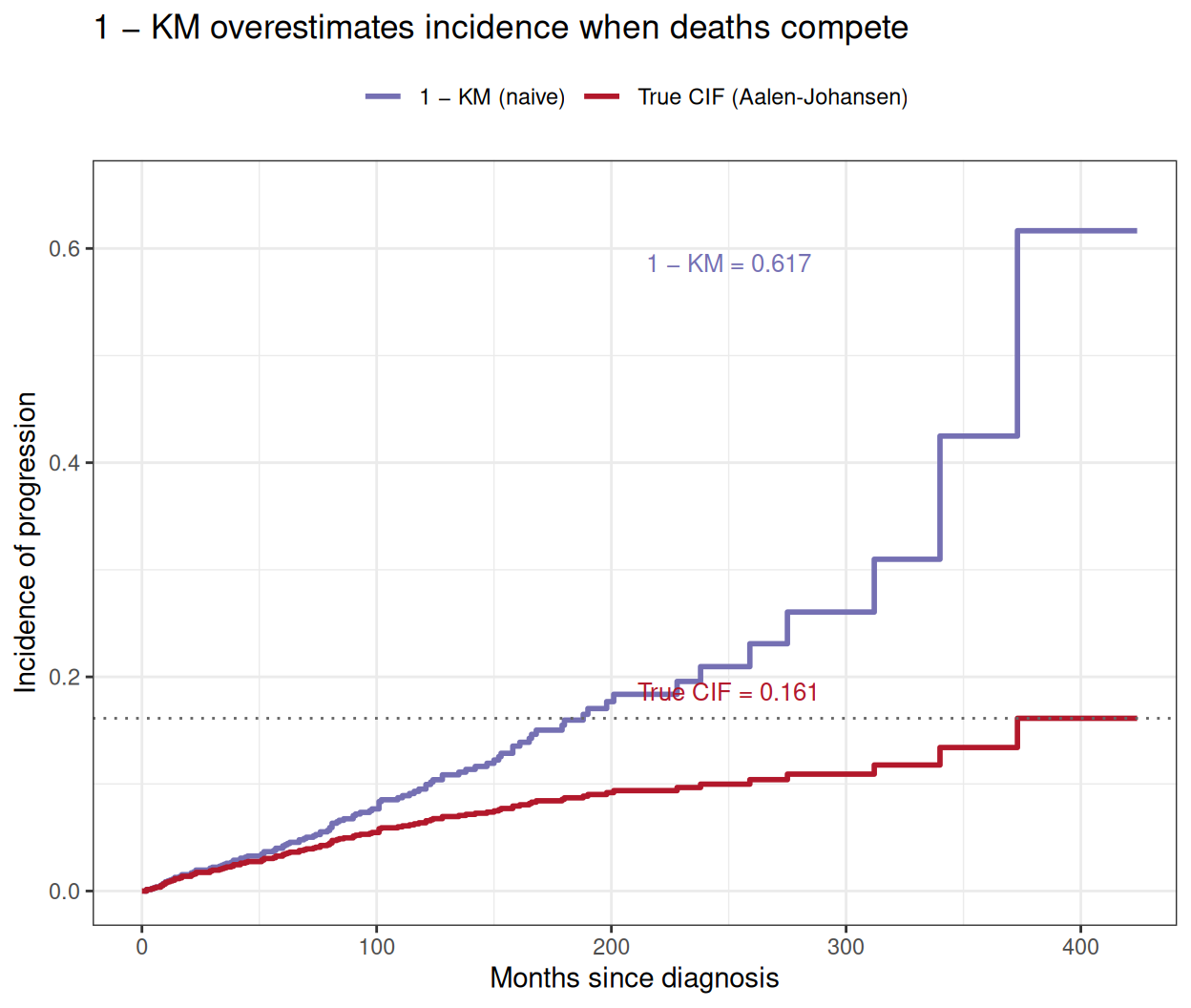
The naive curve rises almost four times above the truth by 20 years. Whenever a competing event is more than a rarity, report Aalen–Johansen CIFs — a Kaplan–Meier curve of the event of interest alone is a common and consequential reviewer catch.
TipPractice tips
- Encode outcomes as a factor with the event of interest first, competing event second, censoring last;
tidycmprsk::cuminc()requires the two-levelSurv(time, factor)syntax. - Report CIFs with confidence intervals and the risk table — readers judge the follow-up, not just the curve.
- Gray’s test compares incidence; the log-rank test on cause-specific survival answers a different question. Pick per the estimand.
- In Fine–Gray models, covariate effects on the subdistribution hazard can have counterintuitive signs (older age appears “protective” against progression because death removes patients first) — interpret against the CIF, not the hazard.
Application
Competing-risk curves are standard in transplantation (relapse vs non-relapse mortality), geriatric oncology (progression vs other-cause death), and device/cardiology studies (arrhythmia vs all-cause death). The panel below mirrors a typical publication layout: (A) CIFs of both outcomes with risk table and (B) the naive 1 − KM versus true CIF comparison.
Reference
[1] Austin PC, Fine JP. Practical recommendations for reporting Fine-Gray model analyses for competing risk data. Stat Med. 2017;36(4):5391-5400. doi:10.1002/sim.7501
[2] Fine JP, Gray RJ. A proportional hazards model for the subdistribution of a competing risk. J Am Stat Assoc. 1999;94(446):496-509. doi:10.1080/01621459.1999.10474144
[3] Sjoberg DD, Fei T. tidycmprsk: competing risks estimation. R package version 1.1.2. 2026. doi:10.32614/CRAN.package.tidycmprsk
[4] Sjoberg DD, Whiting K, Curry M, Lavery JA, Larmarange J. Reproducible summary tables with the gtsummary package. R J. 2021;13:570-580. doi:10.32614/RJ-2021-053 (ggsurvfit builds on gtsummary)
[5] Kyle RA, Therneau TM, Rajkumar SV, et al. A long-term study of prognosis in monoclonal gammopathy of undetermined significance. N Engl J Med. 2002;346(8):564-569. doi:10.1056/NEJMoa011332