# Installing necessary packages
if (!requireNamespace("UpSetR", quietly = TRUE)) {
  install.packages("UpSetR")
}
if (!requireNamespace("ggupset", quietly = TRUE)) {
  install.packages("ggupset")
}

# Load packages
library(UpSetR)
library(ggupset)Upset Plot
The Upset diagram is similar to the Venn diagram, mainly showing the number of elements in the intersection of different sets. However, when the number of sets in the Venn diagram reaches 5, the readability begins to drop sharply. The Upset diagram can well solve the problem of poor readability of the Venn diagram and can also provide additional statistical information on element properties.
Example
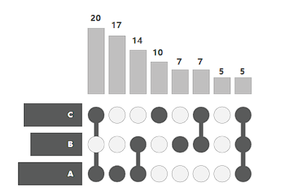
This is the basic style of the Upset graph. The image is divided into three parts. The top part is the histogram of the number of elements in the intersection between different sets, and the left part is the histogram of the number of elements in different sets. The matrix part in the middle is the intersection between the sets, as shown below:
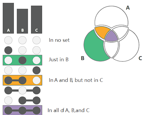
When an element of an intersection exists in a certain set, it is marked with a black dot, otherwise it is marked with a white dot. For example, if the green part is only marked in black in the B set, it means that the column is an element that only exists in B, and so on.
Setup
System Requirements: Cross-platform (Linux/MacOS/Windows)
Programming language: R
Dependent packages:
UpSetR;ggupset
sessioninfo::session_info("attached")─ Session info ───────────────────────────────────────────────────────────────
setting value
version R version 4.6.0 (2026-04-24)
os Ubuntu 24.04.4 LTS
system x86_64, linux-gnu
ui X11
language (EN)
collate C.UTF-8
ctype C.UTF-8
tz UTC
date 2026-05-09
pandoc 3.1.3 @ /usr/bin/ (via rmarkdown)
quarto 1.9.37 @ /usr/local/bin/quarto
─ Packages ───────────────────────────────────────────────────────────────────
package * version date (UTC) lib source
ggupset * 0.4.1 2025-02-11 [1] RSPM
UpSetR * 1.4.0 2019-05-22 [1] RSPM
[1] /home/runner/work/_temp/Library
[2] /opt/R/4.6.0/lib/R/site-library
[3] /opt/R/4.6.0/lib/R/library
* ── Packages attached to the search path.
──────────────────────────────────────────────────────────────────────────────Data Preparation
- The
moviesdataset was created by the GroupLens lab and Bilal Alsallakh; themutationsdataset was originally created by the TCGA consortium and represents the mutational landscape of 100 common gene mutations in 284 glioblastoma multiforme tumors. - Both datasets are included in the UpSetR package
# UpSetR can accept three formats of data. The first is a list with named vectors (see listInput variable), the second is an expression vector (see expressionInput variable), and the third is a data frame consisting of 0,1 (see movies and mutations variables)
# Reading CSV data
# The list format requires each vector in the list to be a set. UpSetR requires each set to be named, and the elements in the vector are members of the corresponding set. When using the upset function to draw, you need to use the fromList function to convert the list data format.
listInput <- list(one = c(1, 2, 3, 5, 7, 8, 11, 12, 13), two = c(1, 2, 4, 5, 10), three = c(1, 5, 6, 7, 8, 9, 10, 12, 13))
# The expression format accepts a vector of expressions. The elements of the expression vector are the names of the sets in the intersection (separated by &), and the numeric elements in the intersection. When using the upset function to draw, you need to use the fromExpression function to convert the list data format.
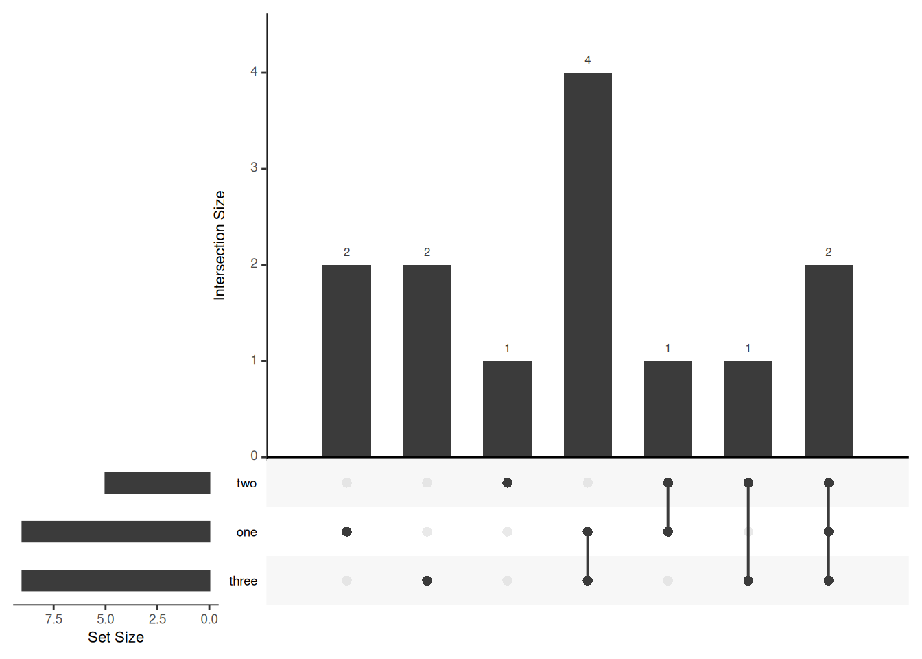
expressionInput <- c(one = 2, two = 1, three = 2, `one&two` = 1, `one&three` = 4, `two&three` = 1, `one&two&three` = 2)
# In the data frame format, each column is a set and each row is an element. The data frame is required to consist of 0 and 1, which respectively indicate whether the element exists in the set. When a column has a value other than 0 or 1, the column is considered to be an attribute of the element.
movies <- read.csv( system.file("extdata", "movies.csv", package = "UpSetR"), header=T, sep=";" )
mutations <- read.csv( system.file("extdata", "mutations.csv", package = "UpSetR"), header=T, sep = ",")Visualization
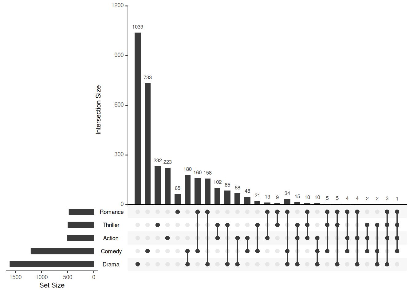
1. Basic Upset Plot
This basic Upset graph shows the number of movies that contain different elements.
# Use the above three data types to draw the Upset graph
upset(fromList(listInput))
upset(fromExpression(expressionInput))
upset(movies)
Tip
Key Parameters: nsets
The nsets parameter determines how many sets are used to draw the UpSet graph, and defaults to 5 when not set.
# Set nset to 6 and use the mutations dataset
upset(mutations, nsets = 6)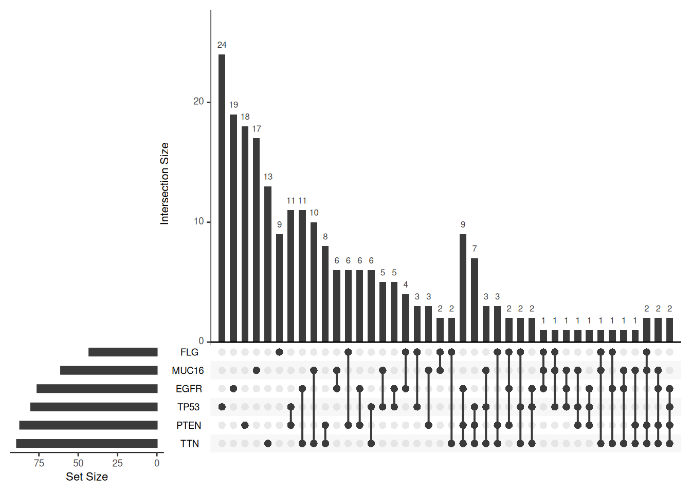
nsets
This graph uses the six most mutated genes to show the number of glioblastoma multiforme tumors that contain different mutations.
Tip
Key Parameters: order.by
The order.by parameter determines the order in which the intersections in the UpSet graph are sorted. If not set, the order is based on the number of sets intersected. If set to “degree”, the order is based on the number of elements in the intersection. If set to “freq”, the order is based on the size of the intersection.
# Three different order.by settings, using the mutations dataset
upset(mutations)
upset(mutations, order.by = "degree")
upset(mutations, order.by = "freq")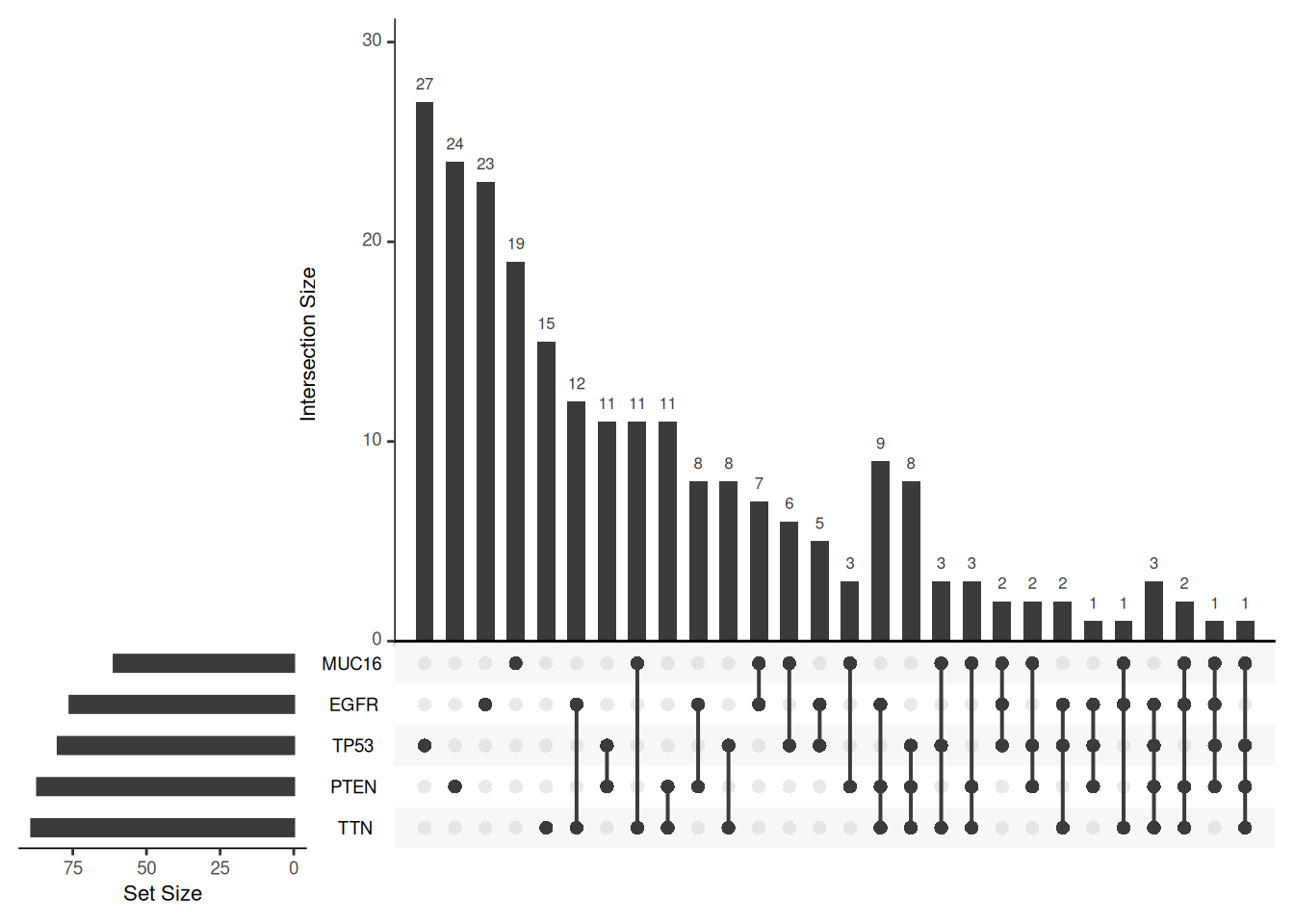
order.by
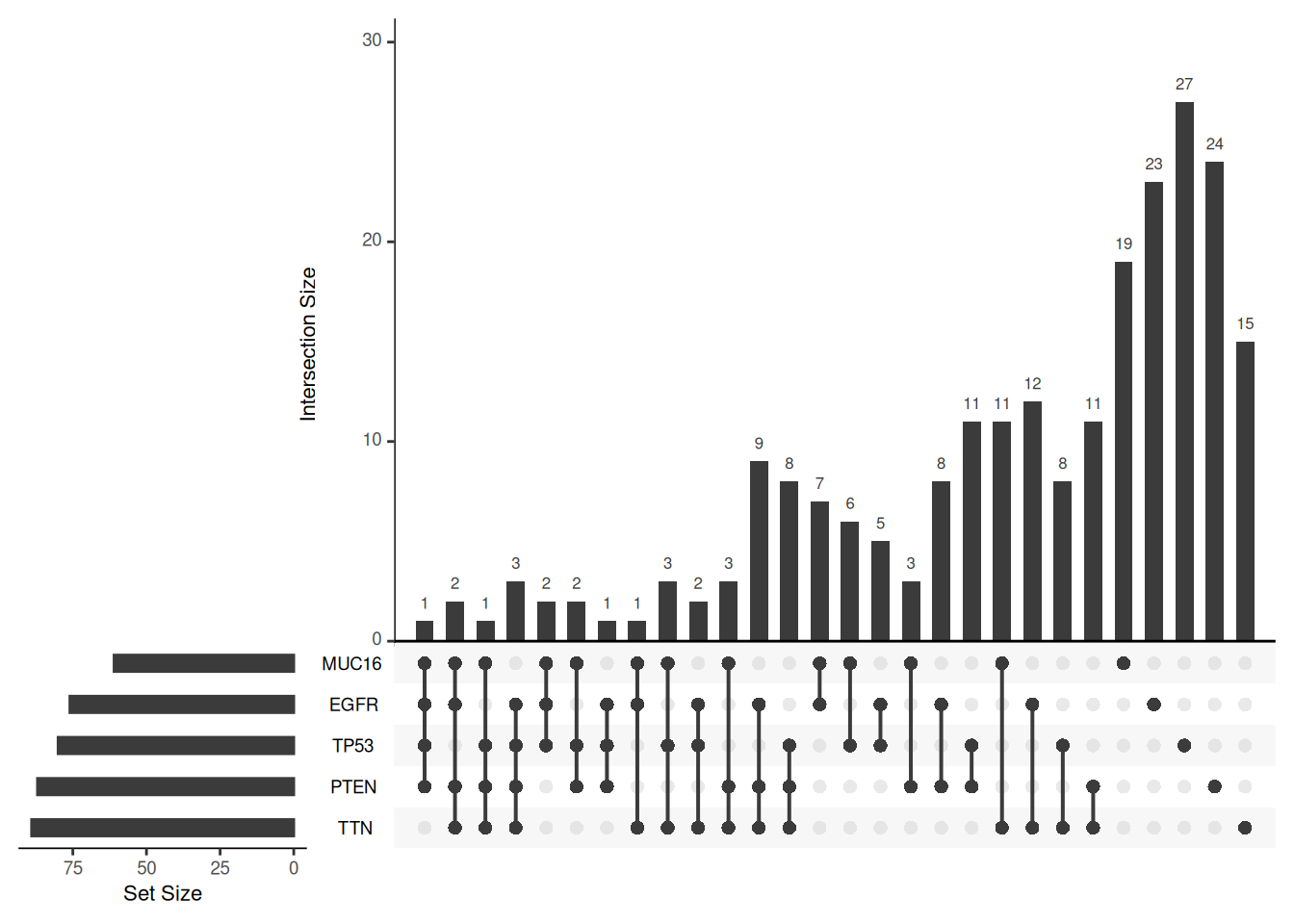
order.by
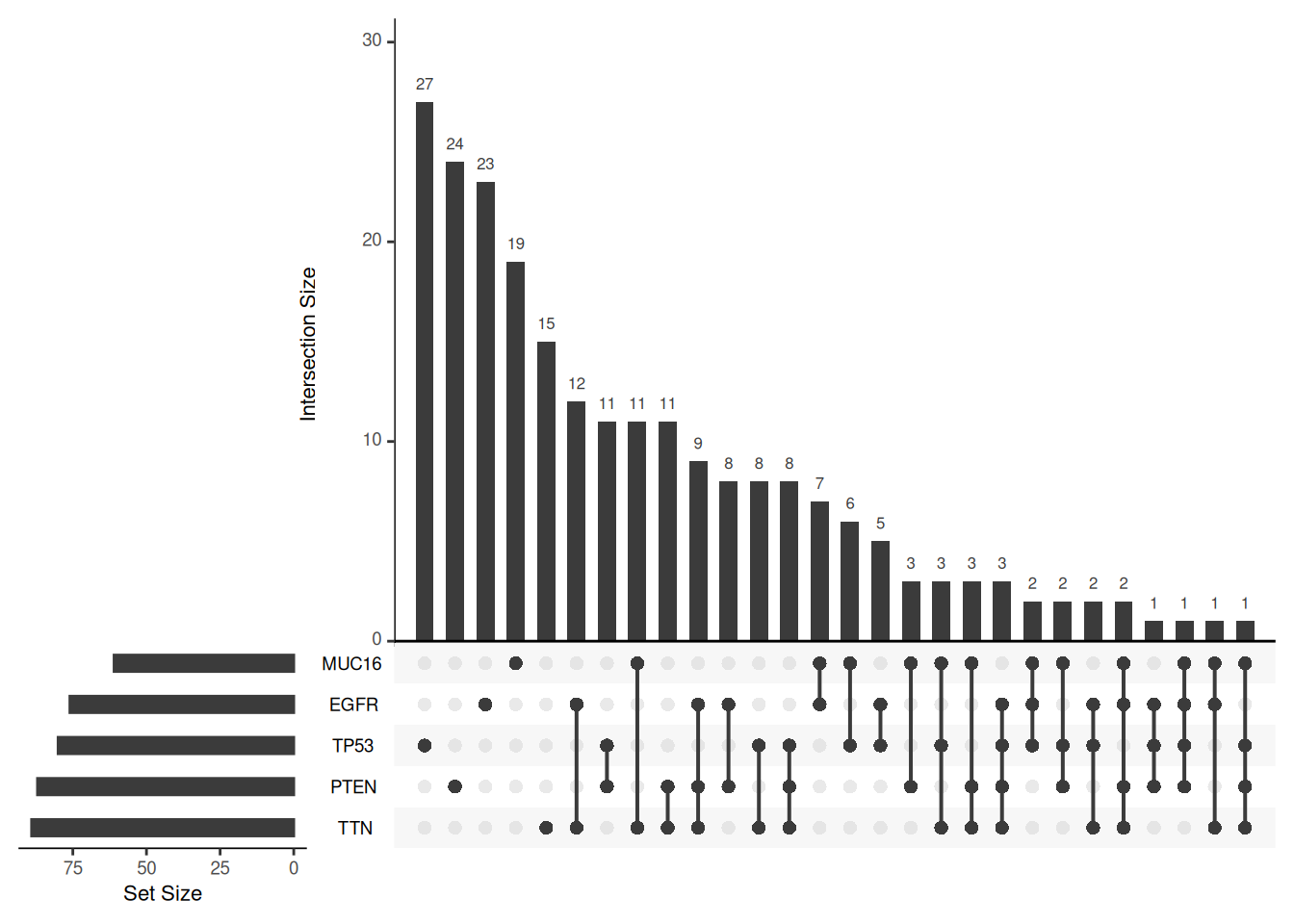
order.by
Tip
Key Parameters: sets
The sets parameter can be used to specify the sets to be plotted. If not set, the nsets sets with the most elements are taken. In addition, the keep.order parameter can keep the order of the set histogram consistent with the order of the sets input.
# Specify "TTN", "NF1", "FLG", "KEL" as the target set, and keep the order of the set bar graph consistent with the sets parameter
upset(mutations, sets = c("TTN","NF1","FLG","KEL"), keep.order = T)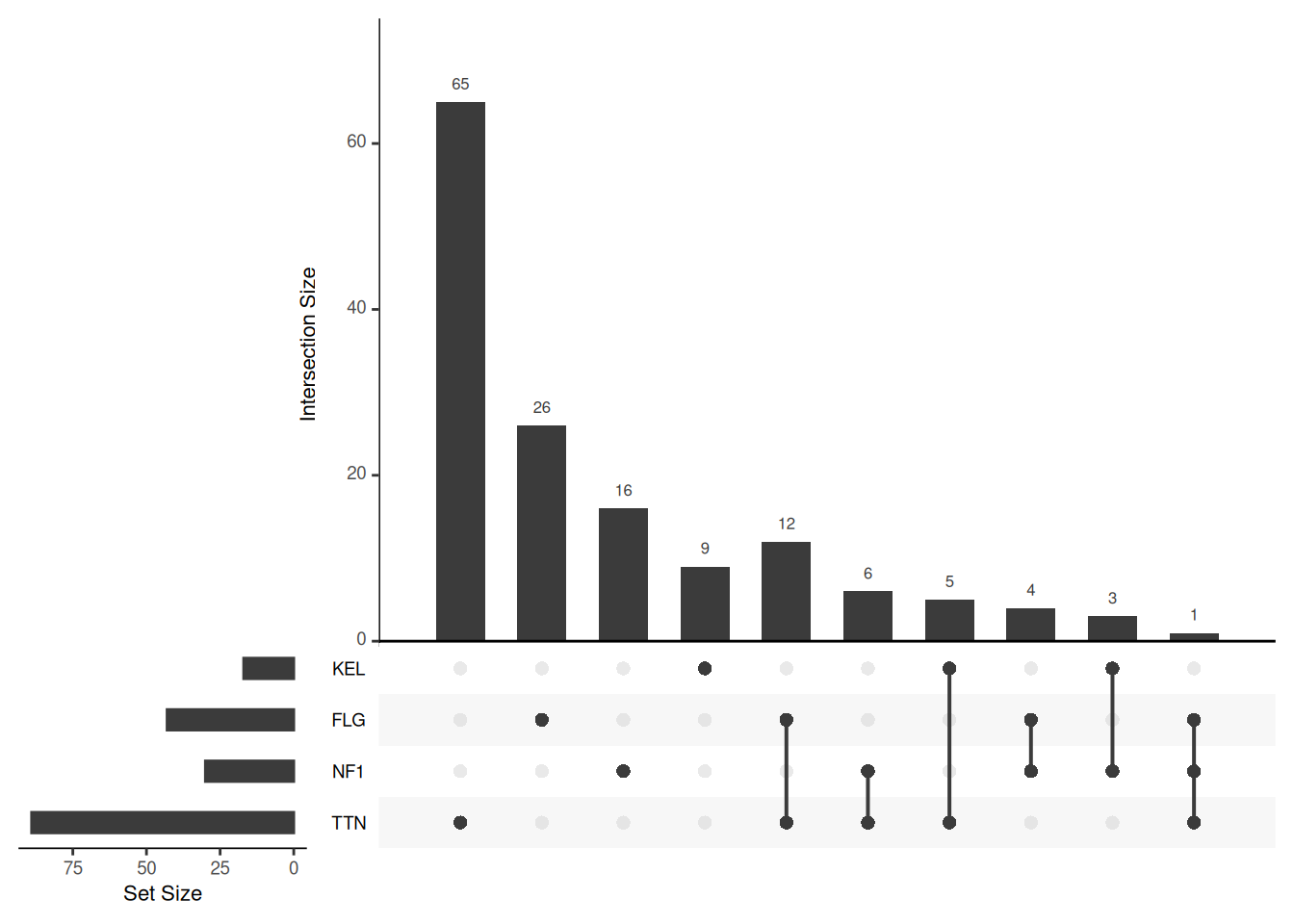
sets
Tip
Key Parameters: empty.intersections
The empty.intersections parameter is set to “NULL” by default, in which case empty intersections are not displayed. When set to any parameter, empty intersections are displayed.
# Show Empty Intersections
upset(mutations, sets = c("TTN","NF1","FLG","KEL"), keep.order = T, empty.intersections=T)empty.intersections
Tip
Key Parameters: decreasing
The decreasing parameter setting can reverse the direction of order.by or keep.order. When there are multiple sorting directions to control, enter a vector with multiple elements, such as “c(T,F)”
# Reverse sort direction
upset(mutations, sets = c("TTN","NF1","FLG","KEL"), keep.order = T, decreasing = c(T, T))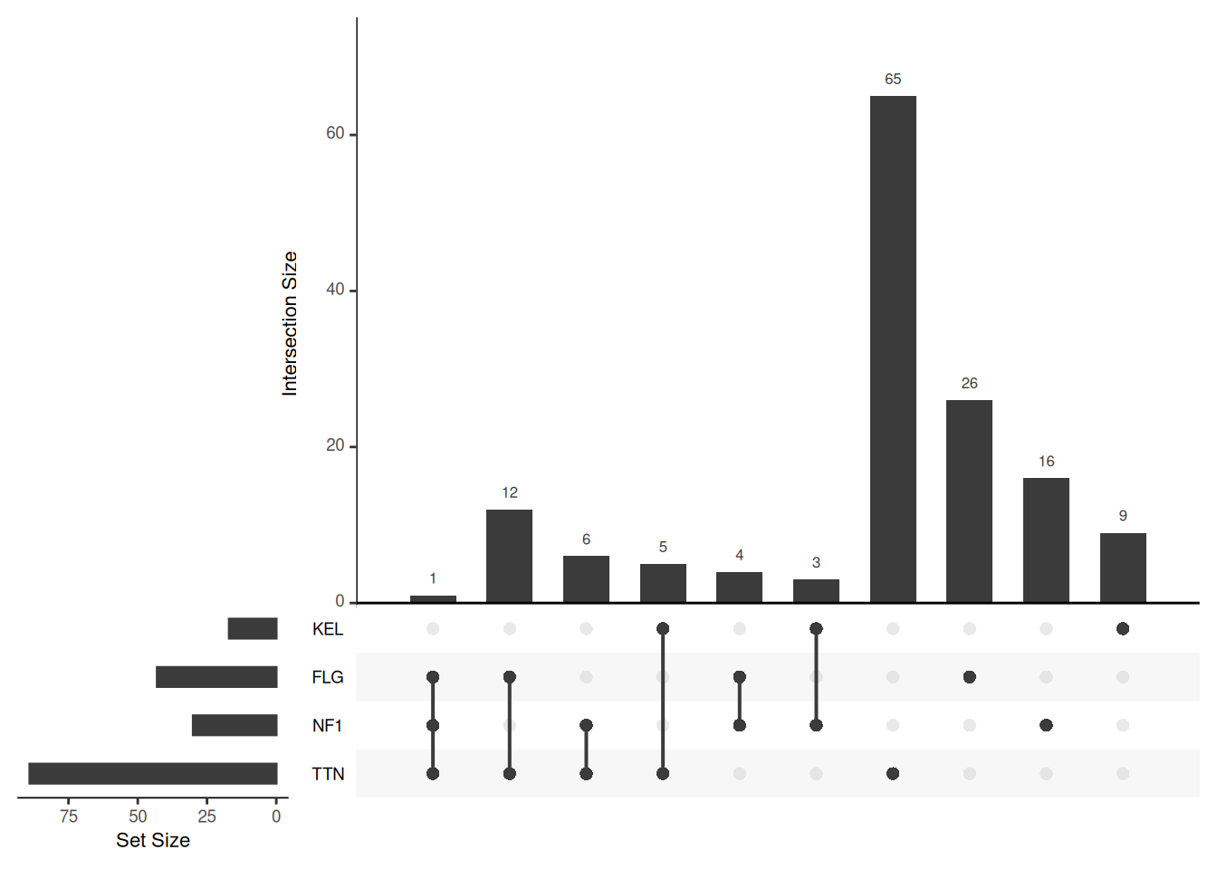
decreasing
2. Personalized Upset Plot
In terms of image ratio, the default value of the mb.ratio parameter is “c(0.7, 0.3)”, which can specify the ratio between the intersection bar graph and the intersection matrix dot graph. You need to input a vector containing two elements, which represent the ratio of the height of the bar graph and the height of the matrix dot graph to the height of the whole image.
upset(mutations, mb.ratio=c(0.5,0.5))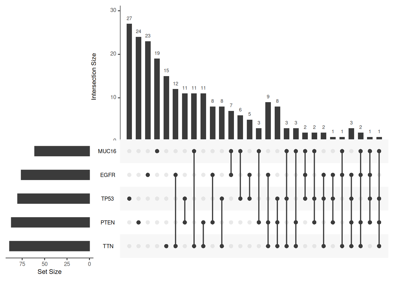
mb.ratio
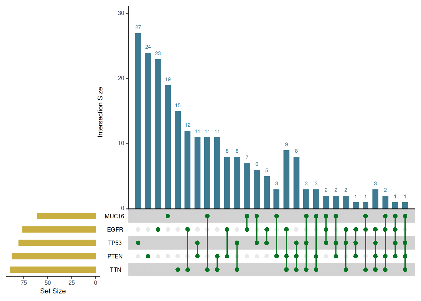
In terms of image color, the UpSetR package provides multiple parameters to set the color of different parts of the Upset image:
upset(mutations,
      shade.color = "#4C4C4C", # Color of the intersection matrix point shadow
      matrix.color = "#067522", # Colors of points and lines in the matrix
      main.bar.color = "#3E7B92", # Color of the histogram of the number of intersection elements
      sets.bar.color = "#C9AE42" # Color of the collection quantity bar chart
)
If you want to highlight certain intersections, you need to use the queries parameter provided by the UpSetR package. The queries parameter requires an input list list, which contains at least one sub-list. Each sub-list needs to contain the following fields: query, params, color, active, and query.name.
- query can be entered as intersects or elements, the effect is the same
- params specifies a subset, the input is also a list, the elements in the list can be the names of the sets, and multiple elements represent the intersection of these elements.
- color is the color that will be represented on the plot. If no color is provided, a color will be selected from the UpSetR default palette.
- active determines how the query will be represented on the plot. If active is TRUE, the cross-size bars will be overlaid by the bars representing the query. If active is FALSE, a jitter point will be placed on the intersecting size bars.
- query.name is the name of the current highlighted set, and the query.legend parameter needs to be used to specify the legend position. query.legend can be entered as “top” or “bottom”
upset(mutations, sets = c("TTN","NF1","FLG","KEL"), keep.order = T,
      query.legend = "top",
      queries = list(list(query = intersects, params = list("TTN"), active = T, query.name = "NAME"),
                     list(query = elements, params = list("TTN","NF1"))))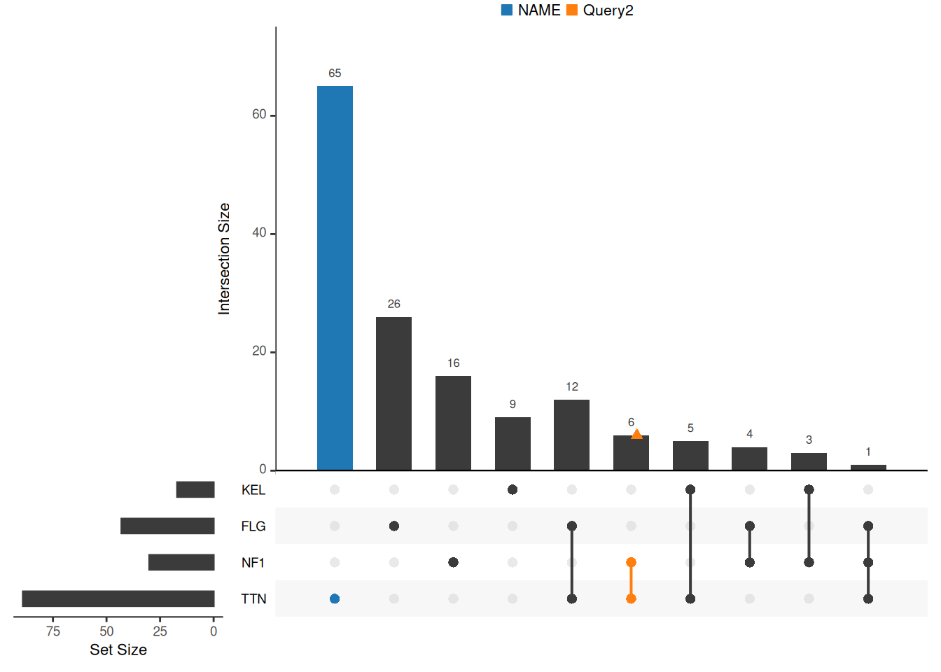
queries
There are also multiple parameters that can be adjusted for image labels and fonts:
upset(mutations,
      number.angles = 30, # The tilt angle of the numbers above the intersection bar graph
      point.size = 2, # The size of the points in the matrix
      line.size = 1, # Size of the lines in the matrix
      sets.x.label = "NAME1", # Axis labels for a collection of bar charts
      mainbar.y.label = "NAME2", # Axis labels for intersection bar chart
      text.scale = c(1.3, 1.3, 1, 1, 1.2,1)) # Text size settings, corresponding to the axis labels of the intersection bar chart, the numbers of the intersection bar chart, the axis labels of the set bar chart, the numbers of the set bar chart, the name of the set, and the numbers above the intersection bar chart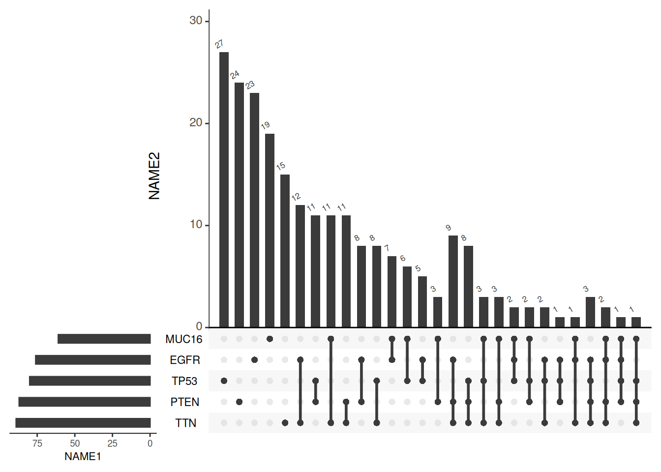
3. Advanced Upset Plot
Sometimes you need to display some properties of the elements in the collection, such as showing the distribution of movies released in 1995 in different intersections. You also need to use the queries parameter. Enter a column name that records the release years of different movies and 1995 in the params field to highlight the distribution of movies released in 1995.
upset(movies, sets = c("Action", "Adventure", "Children", "War", "Noir"),
      queries = list(list(query = elements, params = list("ReleaseDate",1995), active = T)))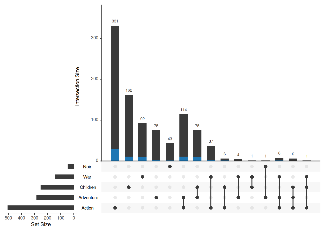
If it is a compound condition, such as highlighting only action movies released in 1995, you can introduce an additional expression parameter to further restrict the query condition.
upset(movies, sets = c("Action", "Adventure", "Children", "War", "Noir"),
      queries = list(list(query = intersects, params = list("Action"), active = T)),
      expression = "ReleaseDate == 1995")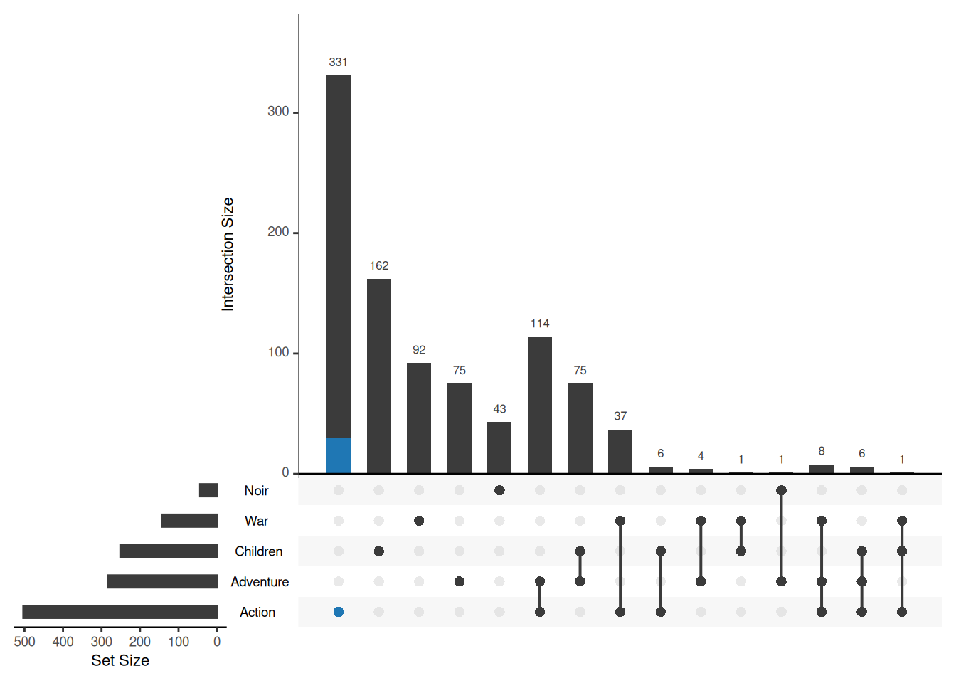
expression
The above method is limited to discrete variables, but the attributes of elements may also include continuous variables. For continuous variables, it is recommended to use custom functions for querying. The following code can be used to highlight elements whose Watches attribute is greater than 100:
Myfunc <- function(row, num) {
  data <- row["Watches"] > num
}
upset(movies, sets = c("Action", "Adventure", "Children", "War", "Noir"),
      queries = list(list(query = Myfunc, params = list(100), active = T)))
UpsetR also supports drawing other types of images at the same time, including histograms, scatter plots, and density plots. The first two need to be drawn using the attribute.plots parameter, and the boxplot needs to be drawn using the boxplot.summary parameter. The boxplot is not compatible with the other three types of images. attribute.plots contains the following sub-parameters:
-
gridrows: Specifies the extent of the plot window to make room for attribute plots. UpSetR plots are based on a 100x100 grid layout. For example, if gridrows is set to 50, the new grid layout will become 150x100, with 1/3 of the area used to place attribute plots. -
plots: Receives a list of parameters including plot, x, y (if applicable), and queries.- plot: is a function that returns a ggplot object, which can be input to histogram or scatter_plot.
- x: defines the x-axis aesthetic mapping used in ggplot (input as a string).
- y: defines the y-axis aesthetic mapping used in ggplot (input as a string).
- queries: controls whether to overlay query results on the property map. If TRUE, the property map will be overlaid with query data; if FALSE, query results will not be shown in the property map.
-
ncols: specifies how the attribute graph is arranged in the space reserved by gridrows. For example:- If two attribute graphs are input and ncols=1, the two graphs are arranged one above the other.
- If two attribute graphs are input and ncols=2, the two graphs are displayed side by side.
upset(movies, sets = c("Action", "Adventure", "Children", "War", "Noir"),
      queries = list(list(query = intersects, params = list("War"), active = T),
                     list(query = elements, params = list("Noir"))),
      attribute.plots=list(gridrows = 100,
                           ncols = 1,
                           plots = list(list(plot=histogram,
                                             x="AvgRating",
                                             queries=T),
                                        list(plot = scatter_plot,
                                             y = "AvgRating",
                                             x = "Watches",
                                             queries = T)
                                        )
                           )
      )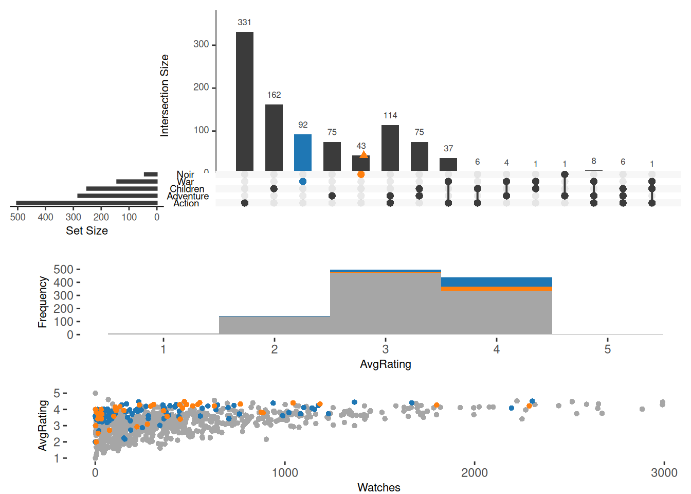
attribute.plots
boxplot.summary is relatively simple, just specify the column name to which the element belongs:
upset(movies, sets = c("Action", "Adventure", "Children", "War", "Noir"),
      queries = list(list(query = intersects, params = list("War"), active = T),
                     list(query = elements, params = list("Noir"))),
      boxplot.summary = c("AvgRating", "ReleaseDate"))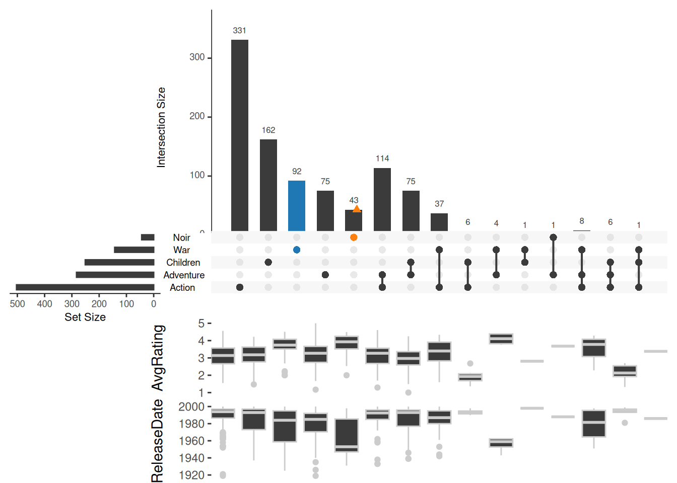
boxplot.summary
4. Biological Data Example
The dataset uses the df_complex_conditions dataset in the ggupset package
# Formatting
df <- df_complex_conditions
df$"T8" <- ifelse(df$Timepoint==8,1,0)
df$"T24" <- ifelse(df$Timepoint==24,1,0)
df$"T48" <- ifelse(df$Timepoint==48,1,0)
df$KO <- ifelse(df$KO=="TRUE",1,0)
df$DrugA <- ifelse(df$DrugA=="Yes",1,0)
# It should be noted that the UpSetR package does not support tibble data frames and needs to be converted to traditional data frames.
df <- data.frame(df[sample(360,180),c(3,4,1,2,5:7)])  # Here we randomly select half of the data for beauty

# upset plot
upset(df,
      queries = list(list(query = intersects, params = list("DrugA","T48"), active = T)),
      boxplot.summary = c("response"))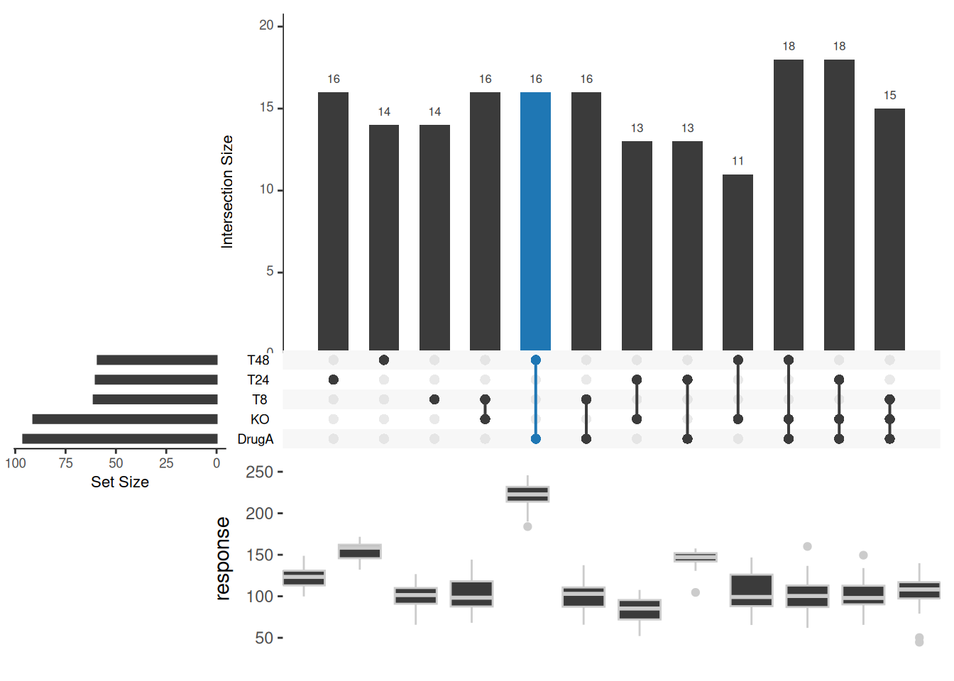
boxplot.summary
This figure shows the response of knockout KO and WT (KO behavior white dots) after or without drug (DrugA) treatment at different times.
Applications
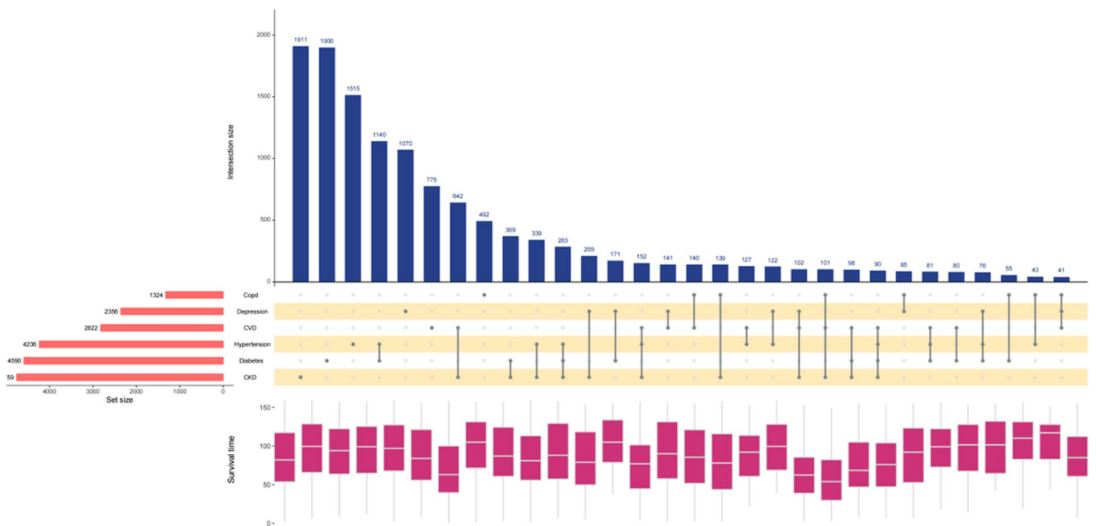
This graph shows the statistics of different diseases in the population and their survival time. [1]
Reference
[1] Peng X, Hu Y, Cai W. Association between urinary incontinence and mortality risk among US adults: a prospective cohort study. BMC Public Health. 2024 Oct 9;24(1):2753. doi: 10.1186/s12889-024-20091-x. PMID: 39385206; PMCID: PMC11463129.