ComplexHeatmap

Example

The Complex Heatmap is an advanced data visualization tool primarily used to display matrix relationships in multidimensional data. It adds multi-level annotation, cluster analysis, and data splitting capabilities to the basic heatmap. It can more clearly present the inherent structure and relationships of complex data.

Setup

• System Requirements: Cross-platform (Linux/MacOS/Windows)

• Programming language: R

• Dependent packages: ComplexHeatmap, dendextend, tidyr, circlize, gridExtra, pheatmap

# Installing packages
if (!requireNamespace("ComplexHeatmap", quietly = TRUE)) {
  install.packages("ComplexHeatmap")
}
if (!requireNamespace("dendextend", quietly = TRUE)) {
  install.packages("dendextend")
}
if (!requireNamespace("tidyr", quietly = TRUE)) {
  install.packages("tidyr")
}
if (!requireNamespace("circlize", quietly = TRUE)) {
  install.packages("circlize")
}
if (!requireNamespace("gridExtra", quietly = TRUE)) {
  install.packages("gridExtra")
}
if (!requireNamespace("pheatmap", quietly = TRUE)) {
  install.packages("pheatmap")
}

# Load packages
library(ComplexHeatmap)
library(dendextend)
library(tidyr)
library(circlize)
library(gridExtra)
library(pheatmap)

Data Preparation

The data mainly comes from the methylation data of the TCGA database

# data_mat (continuous)
data <- readr::read_csv("https://bizard-1301043367.cos.ap-guangzhou.myqcloud.com/TCGA.BRCA.sampleMap_HumanMethylation27_ch.csv")

data <- as.data.frame(data)
rownames(data) <- data[,1]
data <- data[,-1]

data_TCGA <- na.omit(data[1:20,1:20])

data_TCGA <- as.matrix(data_TCGA)  

# Discrete
discrete_mat = matrix(sample(1:5, 100, replace = TRUE), 10, 10)

Visualization

1. Basic ComplexHeatmap

Continuous variables

Here we take the methylation data of the TCGA database as an example

# Continuous variables
Heatmap(data_TCGA , name = "Methylation")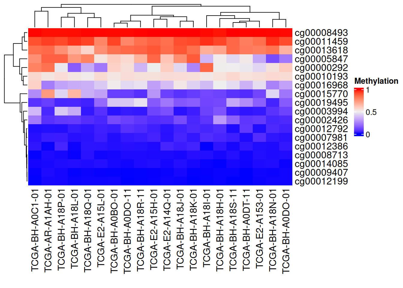

Figure 1: Continuous variables

The figure above shows a complex heatmap of methylation levels, with columns representing gene loci and samples representing behavioral patterns. Red indicates high methylation levels, while blue indicates low methylation levels. The edges represent the results of the cluster analysis.

Discrete variables

Here we take generating data as an example

# Discrete variables
Heatmap(discrete_mat,  name = "mat")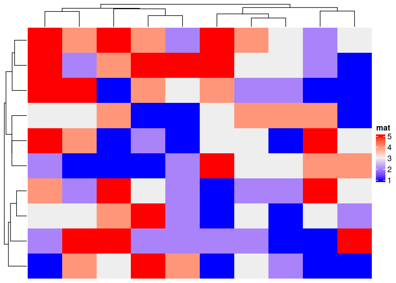

Figure 2: Discrete variables

The figure above is a complex heat map of the generated discrete variables, and the side axes are the results of cluster analysis.

2. Customization

2.1 Color customization

Continuous variables

# Customizing the color of continuous variables
col_fun = colorRamp2(c(0, 0.5, 1),  # Set the cutoff point
                     c("blue", "white", "pink")) 
Heatmap(data_TCGA, name = "Methylation", col = col_fun, 
              column_title = "Custom three-segment color")

Figure 3: Customizing the color of continuous variables

# Customizing the color of continuous variables
Heatmap(data_TCGA, name = "Methylation", col = rev(rainbow(10)), 
        column_title = "Creating a color vector")

Figure 4: Customizing the color of continuous variables

Discrete variables

# Customize discrete variable colors
colors <- c(
  "1" = "#BBEDA7",  
  "2" = "#F3D8FA",  
  "3" = "#FFECA1",  
  "4" = "#D9E6F7",  
  "5" = "#EFBEC6"   
)
Heatmap(discrete_mat, name = "mat", col = colors,
        column_title = "Customize discrete variable colors")

Figure 5: Customize discrete variable colors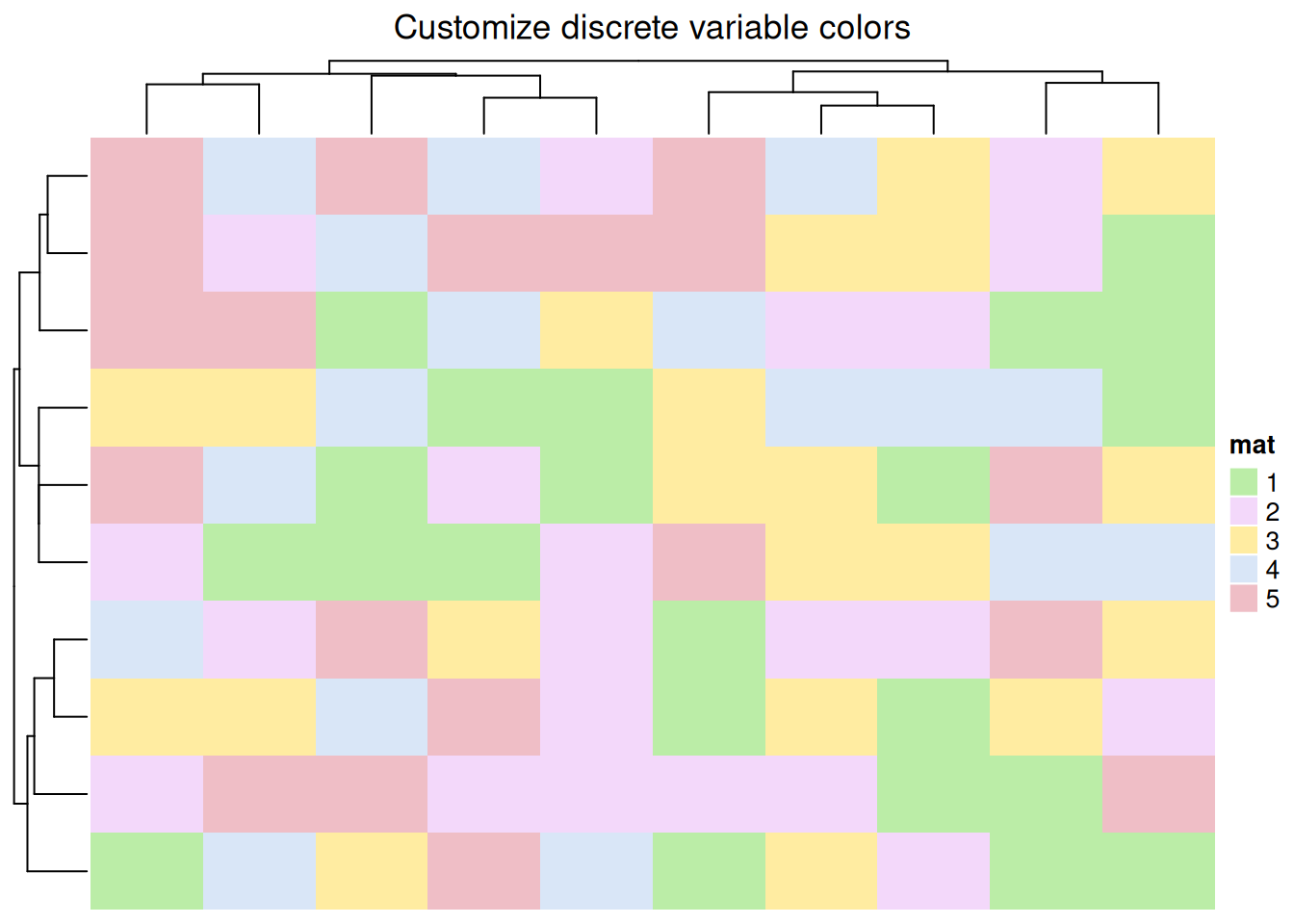

2.2 Border customization

# Border customization
Heatmap(data_TCGA, name = "Methylation", 
        border = "black", # The border value can be FALSE or color
        rect_gp = gpar(col = "white", lwd = 2), # lty line type, lwd line width
        column_title = "Border customization")

Figure 6: Border customization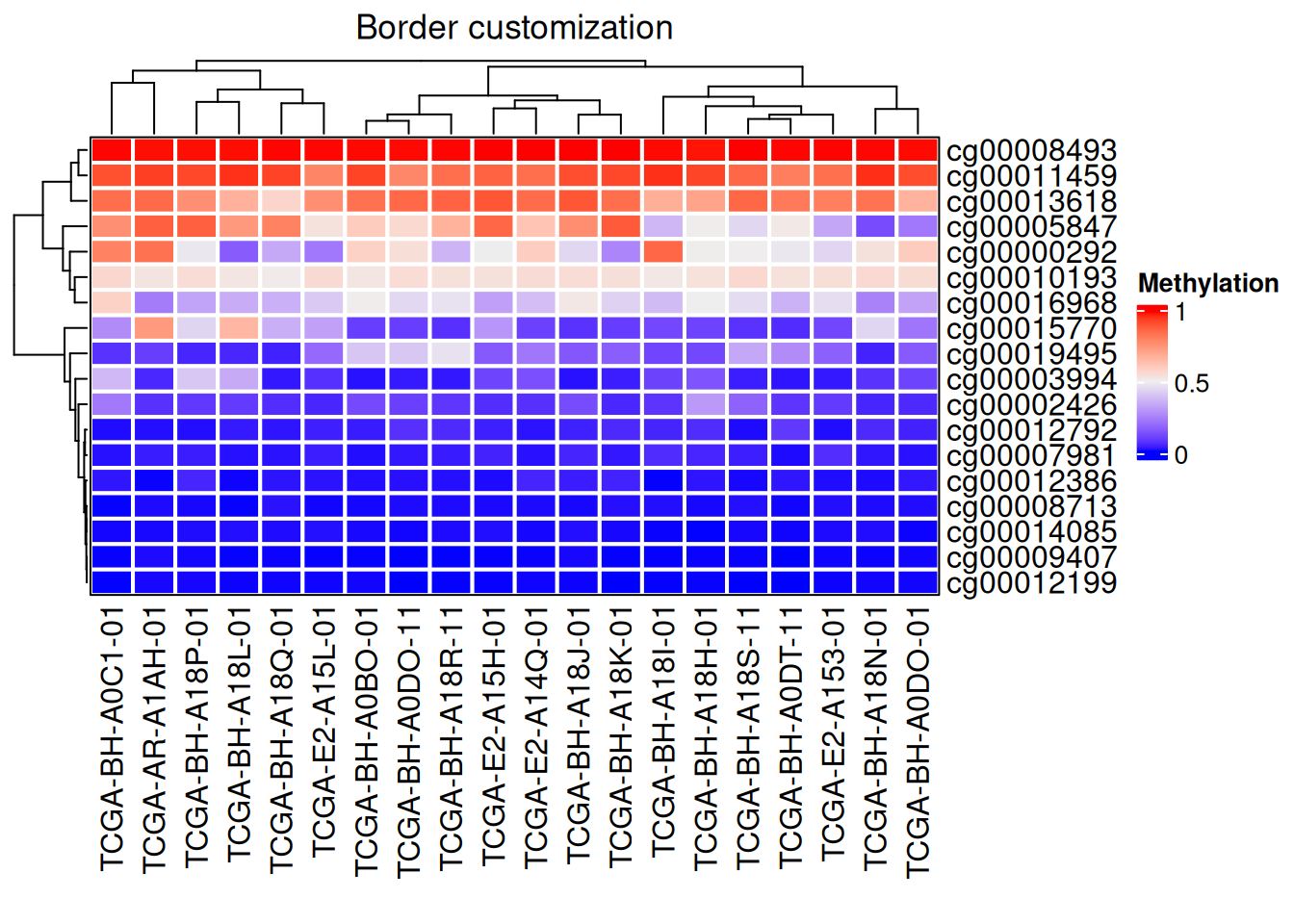

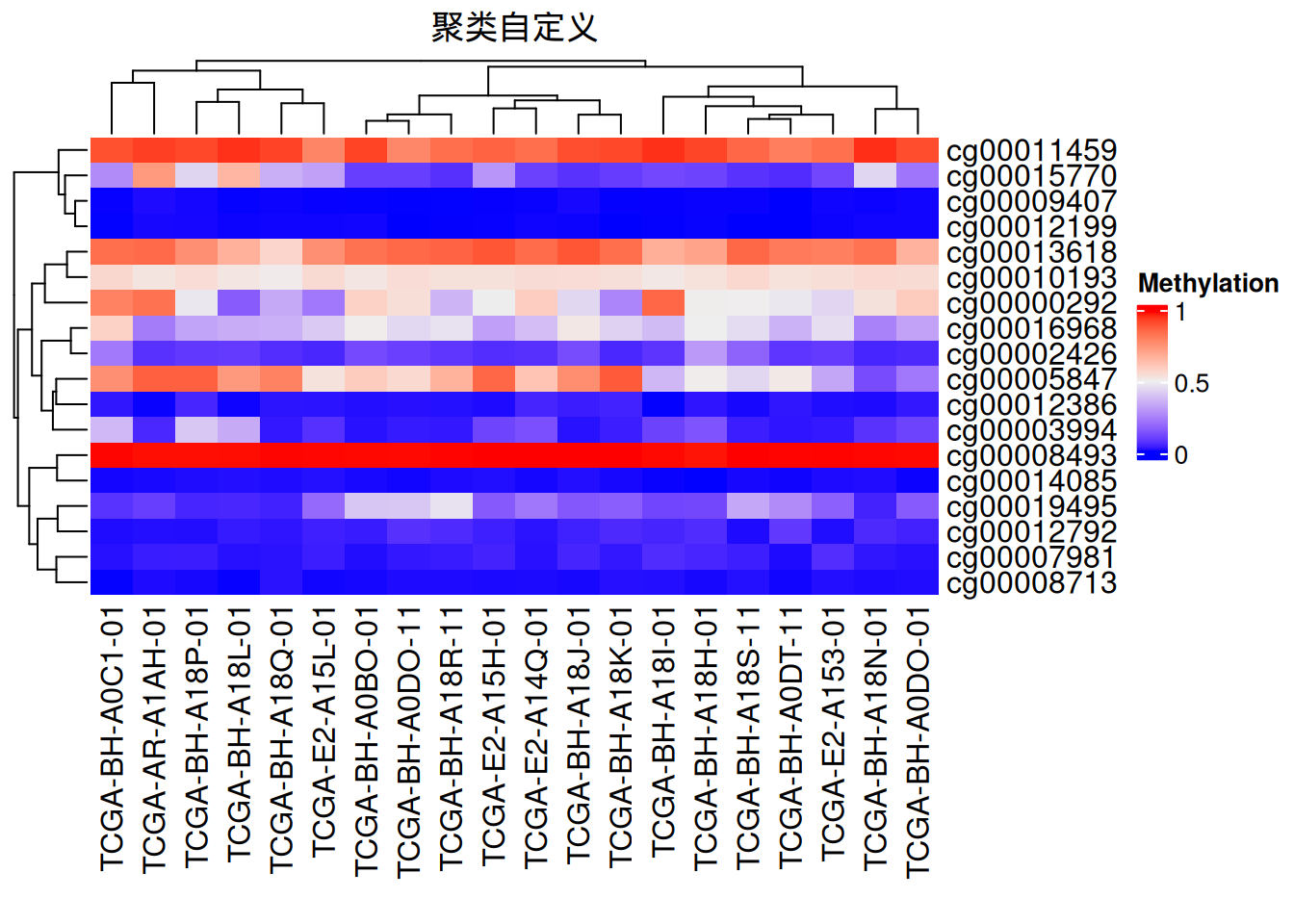
3. Clustering

You can customize clustering methods, dendrogram position, size, etc.

# Clustering
Heatmap(data_TCGA, name = "Methylation", 
       # row_dend_side = "right", 
       # column_dend_side = "bottom", # Adjustable tree view position
        column_dend_height = unit(1, "cm"), 
        row_dend_width = unit(1, "cm"), # Adjustable dendrogram distance
        column_title = "聚类自定义",
        clustering_distance_rows = "pearson", # Clustering method, you can set your own function
      # show_parent_dend_line = FALSE  # Can hide dotted lines
        ) 

Figure 7: Clustering

Dendrogram rendering

We also use the dendextend package to color the dendrogram

# Dendrogram rendering
row_dend = as.dendrogram(hclust(dist(data_TCGA)))
row_dend = color_branches(row_dend, k = 2)  # Generate branches
# Numbers indicate the number of colors
Heatmap(data_TCGA, name = "Methylation", 
        cluster_rows = row_dend,
      # row_dend_gp = gpar(col = "red")  # Customizable colors are also available
        )

Figure 8: Dendrogram rendering

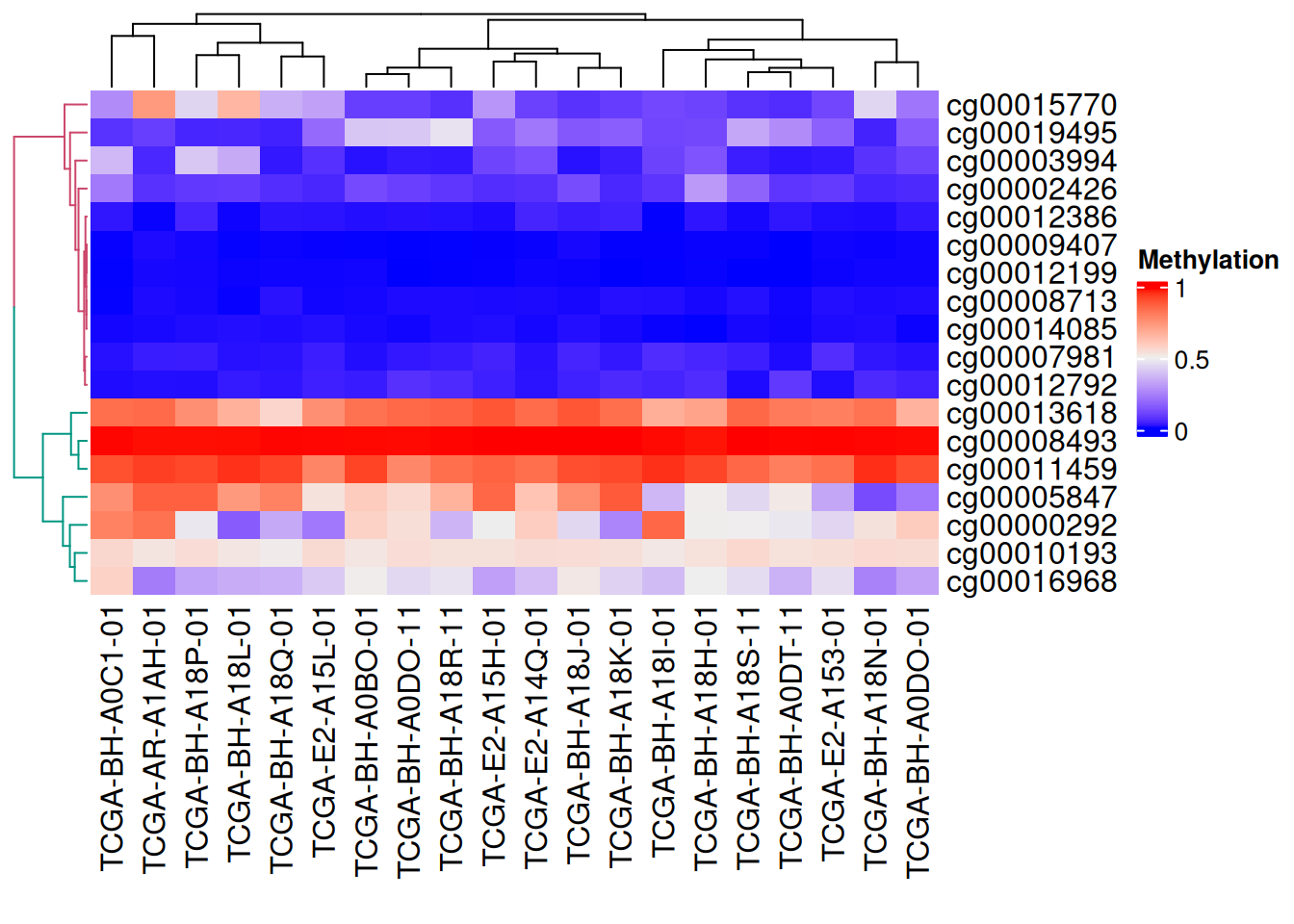
As shown in the figure above, the branches of the tree are different colors.

4. Segmentation

Continuous variables

Use k-means clustering segmentation

# Continuous variable segmentation
Heatmap(data_TCGA, 
        name = "Methylation", 
        row_km = 2,  # Set the number of divisions
        column_km = 3)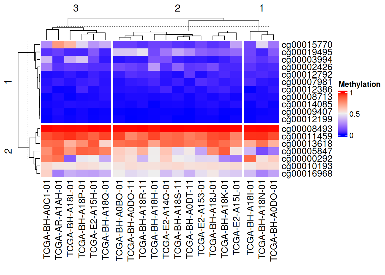

Figure 9: Continuous variable segmentation

Using vector segmentation

# Using vector segmentation
Heatmap(data_TCGA, name = "Methylation", 
        row_split = rep(c("A", "B"), 9), 
        column_split = rep(c("C", "D"), 10))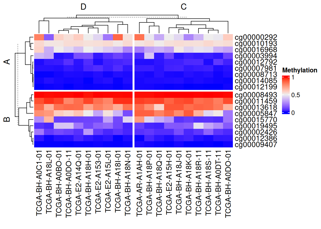

Figure 10: Using vector segmentation

Using matrix segmentation

# Using matrix segmentation
Heatmap(data_TCGA, name = "Methylation", 
        row_split = data.frame(rep(c("A", "B"), 9), 
                               rep(c("C", "D"), each = 9)))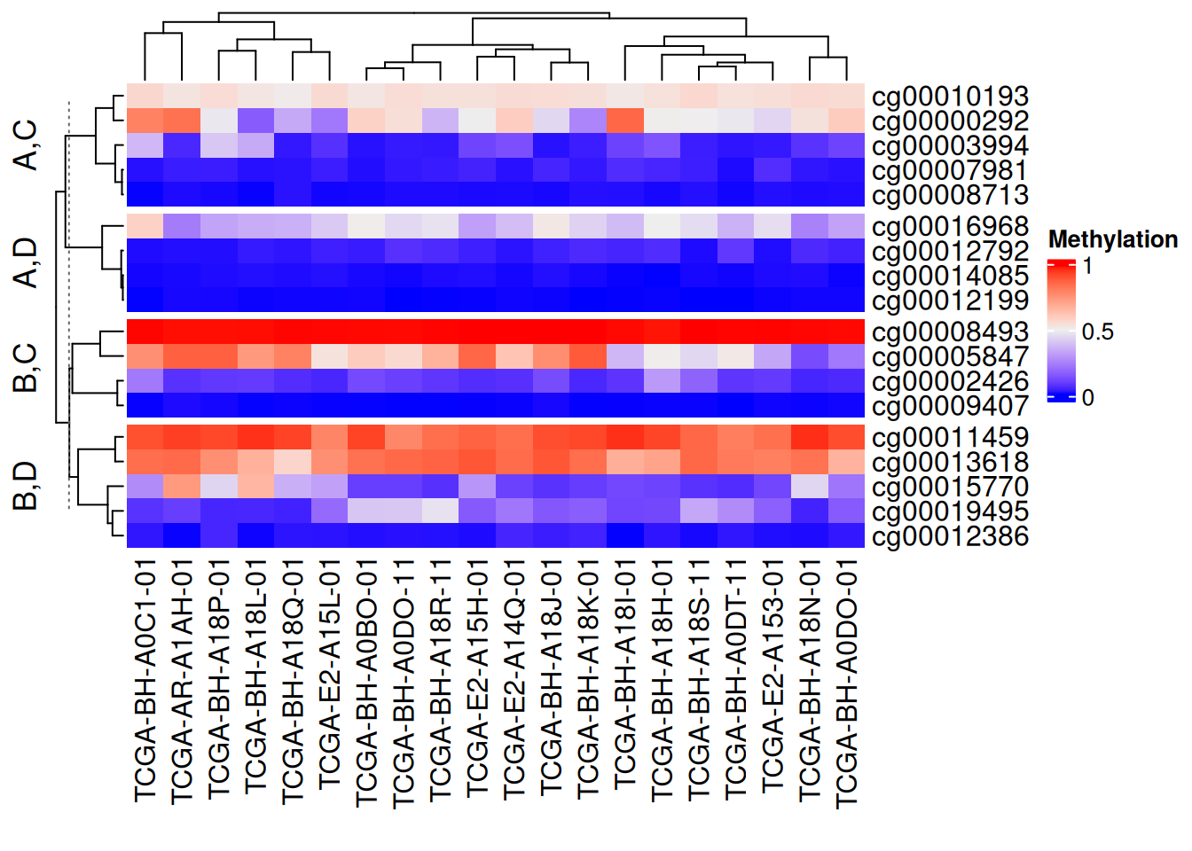

Figure 11: Using matrix segmentation

The above segmentation methods can be used independently in rows and columns. Setting show_parent_dend_line = FALSE can hide the dotted line

Discrete variables

segmentation by specified rows and columns

# segmentation by specified rows and columns
Heatmap(discrete_mat, 
        name = "mat", 
        col = 1:4, 
        row_split = discrete_mat[,1]) # segmentation by the first column in the matrix data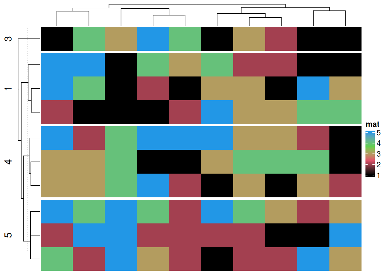

Figure 12: segmentation by specified rows and columns

Parameter segmentation

Titles, clustering parameters, etc. can be segmented based on heatmap segmentation

# Parameter segmentation
Heatmap(data_TCGA, name = "Methylation", 
        row_km = 2, 
        row_title_gp = gpar(col = c("#9A090A", "#0D4B99"), font = 1:2),
        row_names_gp = gpar(col = c("#748901", "#E6AC03"), fontsize = c(10, 12)),
        column_km = 3, 
        column_title_gp = gpar(fill = c("#BFD641", "#FE9900", "#CC6CE7"), font = 1:3),
        column_names_gp = gpar(col = c("#1D6103", "#E08804", "#5E0676"), fontsize = c(10, 12, 8)))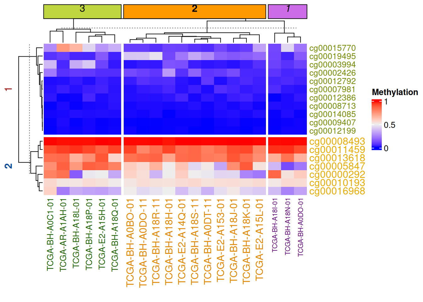

Figure 13: Parameter segmentation

Annotation segmentation

Edge annotations can be segmented based on heatmap segmentation

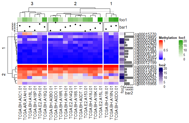
# Annotation segmentation
Heatmap(data_TCGA, name = "Methylation", row_km = 2, column_km = 3,
        top_annotation = HeatmapAnnotation(foo1 = 1:20, bar1 = anno_points(runif(20))),
        right_annotation = rowAnnotation(foo2 = 18:1, bar2 = anno_barplot(runif(18)))
)

Figure 14: Annotation segmentation

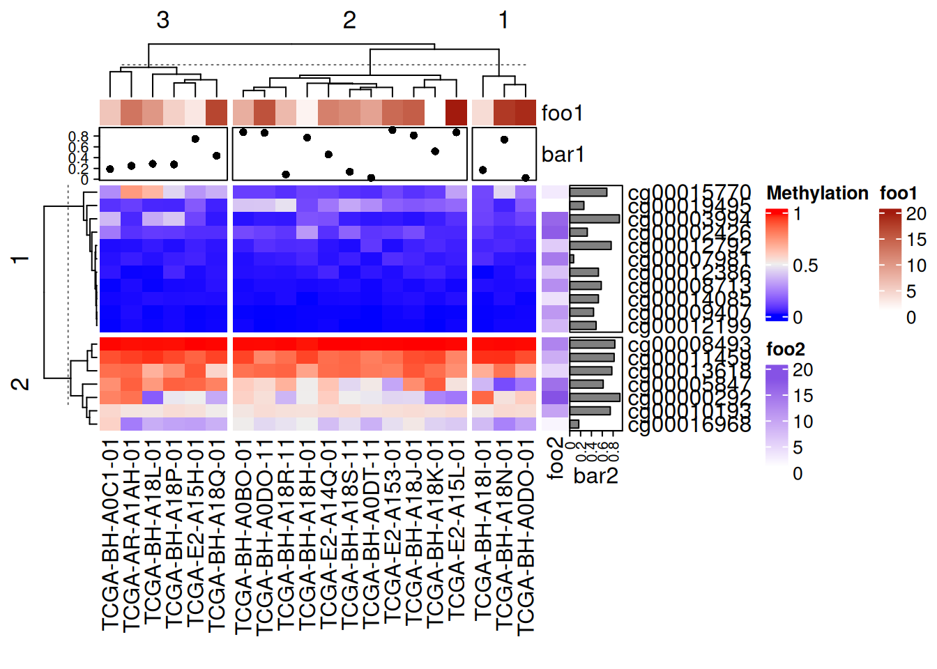
The added point map, heat map, and bar map annotations in the above figure are all segmented with the main heatmap.

5. Add labels

Add data

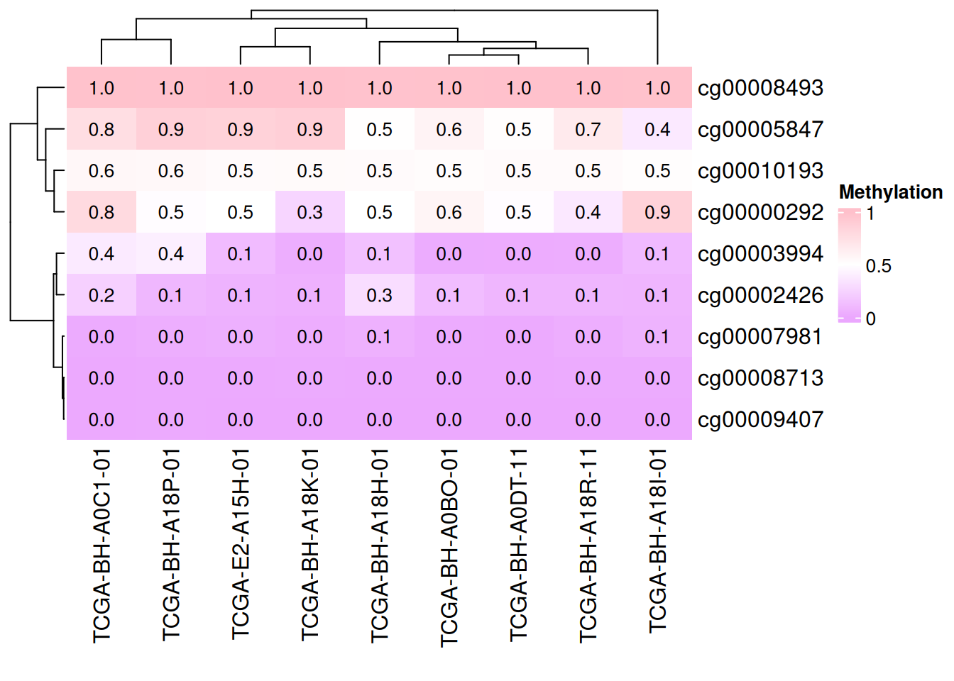
cell_fun accepts a function that is applied to each cell in the heatmap. The function’s arguments are as follows:

• j: Column index (column number).

• i: Row index (row number).

• x, y: Coordinates of the cell center (in the coordinate system of the plotting device).

• width, height: The width and height of the cell.

• fill: The value corresponding to the cell (i.e., the value in the matrix).

# Add data
small_mat = data_TCGA[1:9, 1:9]
col_fun = colorRamp2(c(0, 0.5, 1), c("#EBA7FE", "white", "pink"))
Heatmap(small_mat, name = "Methylation", col = col_fun,
        cell_fun = function(j, i, x, y, width, height, fill) {
          grid.text(sprintf("%.1f", small_mat[i, j]), x, y, gp = gpar(fontsize = 10))
        })

Figure 15: Add data

# Add data
small_mat = data_TCGA[1:9, 1:9]
Heatmap(small_mat, name = "Methylation",  col = col_fun,
        cell_fun = function(j, i, x, y, width, height, fill) {
          if(small_mat[i, j] > 0.5) # Set the display range
            grid.text(sprintf("%.1f", small_mat[i, j]), x, y, gp = gpar(fontsize = 10)) # Add text/value
        })

Figure 16: Add data

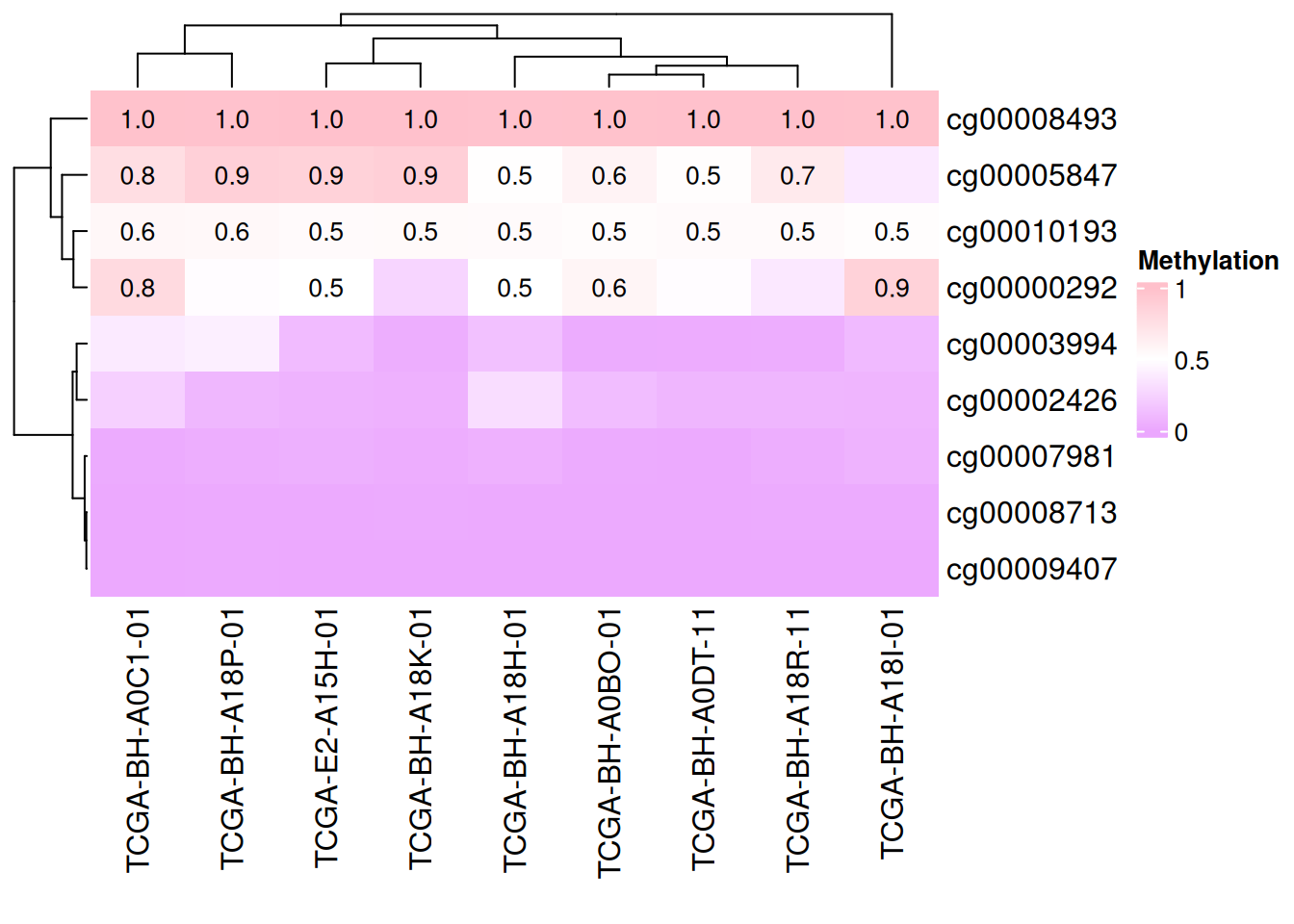
The above figure only shows data with methylation levels greater than 0.5

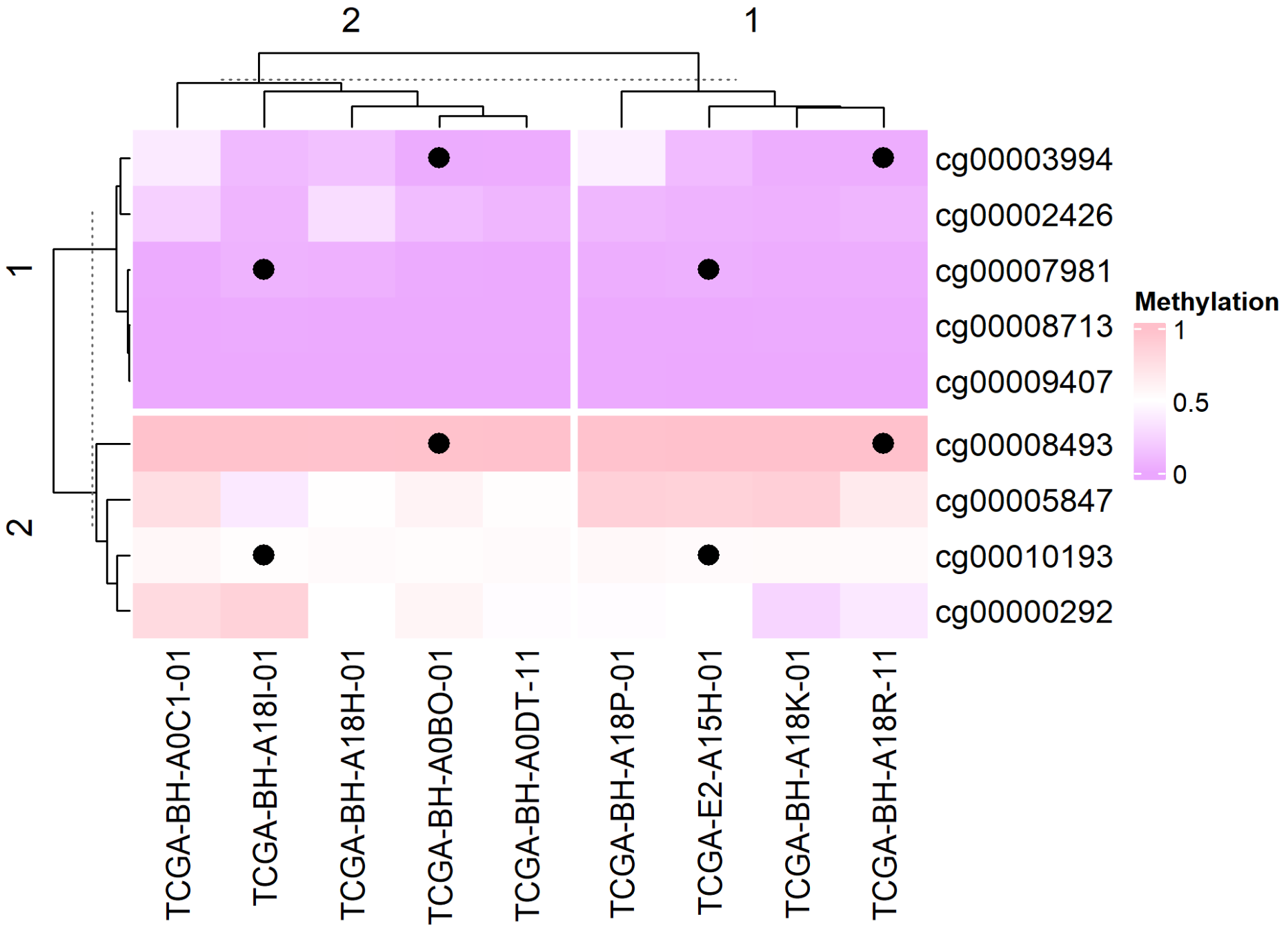
Add graphics

# Add graphics
small_mat = data_TCGA[1:9, 1:9]
Heatmap(small_mat, name = "Methylation", col = col_fun,
        row_km = 2, column_km = 2,
        layer_fun = function(j, i, x, y, w, h, fill) {
          ind_mat = restore_matrix(j, i, x, y)
          ind = unique(c(ind_mat[1, 4], ind_mat[3, 2])) # Positioning, add graphics to each segmentation location
          grid.points(x[ind], y[ind], pch = 16, size = unit(4, "mm")) # Add Point
        }
)

Figure 17: Add graphics

Application

Figure 18: Applications of ComplexHeatmap

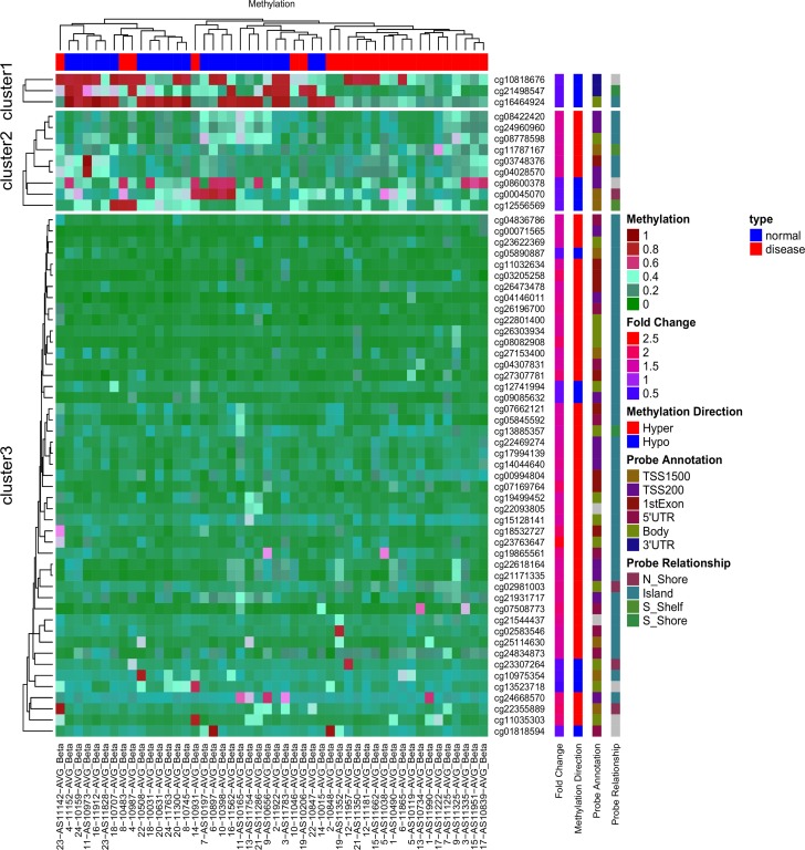
The figure above is an unsupervised hierarchical clustering heatmap of 59 differentially methylated ATG sites in the AVR data [1]. Red indicates high DNA methylation, and green indicates low DNA methylation.

Reference

[1] Radhakrishna U, Albayrak S, Alpay-Savasan Z, Zeb A, Turkoglu O, Sobolewski P, Bahado-Singh RO. Genome-Wide DNA Methylation Analysis and Epigenetic Variations Associated with Congenital Aortic Valve Stenosis (AVS). PLoS One. 2016 May 6;11(5):e0154010. doi: 10.1371/journal.pone.0154010. PMID: 27152866; PMCID: PMC4859473.

[2] Gu, Z. (2016) Complex heatmaps reveal patterns and correlations in multidimensional genomic data. Bioinformatics.Gu, Z. (2022) Complex Heatmap Visualization. iMeta.

[3] Tal Galili (2015). dendextend: an R package for visualizing, adjusting, and comparing trees of hierarchical clustering. Bioinformatics. DOI:10.1093/bioinformatics/btv428

[4] Wickham H, Vaughan D, Girlich M (2024). tidyr: Tidy Messy Data. R package version 1.3.1, CRAN: Package tidyr.

[5] Gu, Z. (2014) circlize implements and enhances circular visualization in R. Bioinformatics.

[6] Auguie B (2017). gridExtra: Miscellaneous Functions for “Grid” Graphics. R package version 2.3, CRAN: Package gridExtra.

[7] Kolde R (2019). pheatmap: Pretty Heatmaps. R package version 1.0.12, CRAN: Package pheatmap.