Interactive Volcano Plot

🤖 AI Skill — Download the Bizard unified skill for your AI assistant ⬇️ Download Skill ZIP

The interactive volcano plot is a visualization tool for differential expression analysis of high-throughput data (e.g., transcriptomics, proteomics). Building upon the traditional volcano plot, it supports mouse hover to view gene information, click to jump to external databases, and provides more flexible threshold settings and color schemes, helping researchers screen and interpret differential analysis results more efficiently.

Example

This is a static preview.

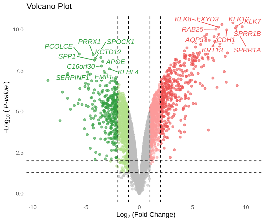
In this volcano plot, the x-axis represents log2FC values and the y-axis represents -log10(P) values. Gray scatter points indicate non-significant genes; light blue and light red points represent genes meeting conventional thresholds (pval_cutoff, logFC_cutoff); dark blue and dark red points represent genes simultaneously meeting strict thresholds (pval_cutoff2, logFC_cutoff2). This color scheme is automatically applied by the FigureYa theme. Hovering over any scatter point displays the gene name, log2(FC), and P.val value; clicking a gene jumps to the GeneCards website. By default, the top 10 up-regulated and top 10 down-regulated genes are labeled.

Setup

• System Requirements: Cross-platform (Linux/MacOS/Windows)

• Programming language: R

• Dependent packages: ivolcano, fanyi, clusterProfiler, org.Hs.eg.db

# Installing necessary packages
if (!requireNamespace("ggplot2", quietly = TRUE)) {
  install.packages("ggplot2")
}
if (!requireNamespace("ivolcano", quietly = TRUE)) {
  install.packages("ivolcano")
}
if (!requireNamespace("fanyi", quietly = TRUE)) {
  remotes::install_github("YuLab-SMU/fanyi")
}
if (!requireNamespace("clusterProfiler", quietly = TRUE)) {
  install.packages("clusterProfiler")
}
if (!requireNamespace("org.Hs.eg.db", quietly = TRUE)) {
  BiocManager::install("org.Hs.eg.db")
}

# Load packages
library(ggplot2)
library(ivolcano)
library(fanyi)
library(clusterProfiler)
library(org.Hs.eg.db)

sessioninfo::session_info("attached")

─ Session info ───────────────────────────────────────────────────────────────
 setting  value
 version  R version 4.6.0 (2026-04-24)
 os       Ubuntu 24.04.4 LTS
 system   x86_64, linux-gnu
 ui       X11
 language (EN)
 collate  C.UTF-8
 ctype    C.UTF-8
 tz       UTC
 date     2026-05-05
 pandoc   3.1.3 @ /usr/bin/ (via rmarkdown)
 quarto   1.9.37 @ /usr/local/bin/quarto

─ Packages ───────────────────────────────────────────────────────────────────
 package         * version    date (UTC) lib source
 AnnotationDbi   * 1.74.0     2026-04-28 [1] Bioconduc~
 Biobase         * 2.72.0     2026-04-28 [1] Bioconduc~
 BiocGenerics    * 0.58.0     2026-04-28 [1] Bioconduc~
 clusterProfiler * 4.20.0     2026-04-28 [1] Bioconduc~
 fanyi           * 0.1.1      2026-05-04 [1] Github (YuLab-SMU/fanyi@26d2454)
 generics        * 0.1.4      2025-05-09 [1] RSPM
 ggplot2         * 4.0.3.9000 2026-05-04 [1] Github (tidyverse/ggplot2@6870419)
 IRanges         * 2.46.0     2026-04-28 [1] Bioconduc~
 ivolcano        * 0.0.5      2026-02-14 [1] RSPM
 org.Hs.eg.db    * 3.23.1     2026-05-04 [1] Bioconductor
 S4Vectors       * 0.50.0     2026-04-28 [1] Bioconduc~

 [1] /home/runner/work/_temp/Library
 [2] /opt/R/4.6.0/lib/R/site-library
 [3] /opt/R/4.6.0/lib/R/library
 * ── Packages attached to the search path.

──────────────────────────────────────────────────────────────────────────────

Data Preparation

We use the built-in easy_input_limma.rds dataset from the ivolcano package, which contains differential analysis results from the human airway epithelial cell airway dataset.

# Load data
f1 <- system.file("extdata/easy_input_limma.rds", package = "ivolcano")
df_limma <- readRDS(f1)
# View dataset
head(df_limma)

       X    logFC   AveExpr         t      P.Value    adj.P.Val        B
1  KLK10 8.778049 10.506750 111.57547 3.802229e-11 1.760315e-07 15.41764
2  FXYD3 7.748971 10.459578 107.27217 4.809044e-11 1.760315e-07 15.29791
3   KLK7 9.138924 10.596380 102.65832 6.252983e-11 1.760315e-07 15.15779
4 SPRR1B 9.646357 10.570985 101.27838 6.779348e-11 1.760315e-07 15.11331
5   KLK8 7.419248  8.592425 100.42890 7.129085e-11 1.760315e-07 15.08531
6 SPRR1A 9.001559 10.692375  98.45984 8.023989e-11 1.760315e-07 15.01850

Note: The input data frame must contain at least three columns: fold change, significance P value, and gene name. Column names can be specified via corresponding parameters.

Visualization

1. Basic Plotting

You can directly draw an interactive volcano plot using the ivolcano function. It outputs an interactive HTML plot by default; set interactive = FALSE to obtain a static ggplot object.

# Basic interactive volcano plot
p <- ivolcano(df_limma,
         logFC_col = "logFC",
         pval_col  = "P.Value",
         gene_col  = "X")

p

Figure 1: Basic interactive volcano plot

Figure 1 shows the most basic interactive volcano plot using default parameters. Mouse hover reveals gene information.

Tip

Key Parameters:

• pval_cutoff/logFC_cutoff: Conventional significance thresholds; genes below these thresholds are classified as non-significant.
• pval_cutoff2/logFC_cutoff2: Stricter thresholds; genes meeting these conditions are assigned darker colors, split into two levels with the FigureYa green-gray-red color scheme automatically applied. If not set, no stratification occurs.
• top_n: Labels the top n most significant up-regulated and down-regulated genes; default is 10.

# Dual thresholds + FigureYa color scheme
p <- ivolcano(df_limma,
         logFC_col    = "logFC",
         pval_col     = "P.Value",
         gene_col     = "X",
         pval_cutoff  = 0.05,
         pval_cutoff2 = 0.01,
         logFC_cutoff  = 1,
         logFC_cutoff2 = 2,
         top_n = 5)

p

Figure 2: Dual thresholds with FigureYa theme coloring

Tip

Key Parameters:

• size_by: Maps scatter point size to a statistic or data column to enhance visual hierarchy. Options include "none" (default), "negLogP", "absLogFC", or any column name in the data frame.
• point_size: Only effective when size_by = "manual", sets point sizes for non-significant (base), moderately significant (medium), and highly significant (large) points.

# Map point size by negLogP
p <- ivolcano(df_limma,
         logFC_col  = "logFC",
         pval_col   = "P.Value",
         gene_col   = "X",
         size_by    = "negLogP")

p

Figure 3: Map point size by -log10(P) value

# Manually specify point sizes by significance level
p <- ivolcano(df_limma,
         logFC_col    = "logFC",
         pval_col     = "P.Value",
         gene_col     = "X",
         pval_cutoff  = 0.05,
         pval_cutoff2 = 0.01,
         logFC_cutoff  = 1,
         logFC_cutoff2 = 2,
         size_by = "manual",
         point_size = list(base = 2, medium = 4, large = 6))

p

Figure 4: Manually specify point sizes by layer (base=2, medium=4, large=6)

Tip

Key Parameters:

• filter: Allows direct filtering of genes to label as a string, e.g., X %in% genes to label a specified gene set. Once filter is specified, the top_n parameter is automatically disabled.

# Label genes with logFC > 8
p <- ivolcano(df_limma,
         logFC_col   = "logFC",
         pval_col    = "P.Value",
         gene_col    = "X",
         pval_cutoff  = 0.05,
         logFC_cutoff  = 1,
         filter = "logFC > 8")

p

Figure 5: Label extremely differential genes (logFC > 8)

2. Click-to-Jump and Rich Information Cards

The onclick_fun parameter in the ivolcano function accepts a function defining the behavior after clicking a scatter point. Built-in functions allow direct jumps to common gene databases.

# Click gene to jump to NCBI
p <- ivolcano(df_limma,
         logFC_col   = "logFC",
         pval_col    = "P.Value",
         gene_col    = "X",
         onclick_fun = onclick_ncbi)

p

Figure 6: Click gene to jump to NCBI

In Figure 6, clicking any gene opens its NCBI page.

Tip

Key Parameters:

• onclick_fun: Built-in jump functions include onclick_genecards, onclick_ncbi, onclick_ensembl, onclick_pubmed, etc.
• onclick_fanyi: Provided by the fanyi package, allows creating custom click-to-display functions based on a gene information data frame.

# Prepare gene summary data
df_limma$entrez <- mapIds(org.Hs.eg.db, keys = df_limma$X,
                    column = "ENTREZID", keytype = "SYMBOL",
                    multiVals = "first")
top_eg <- df_limma$entrez[order(df_limma$P.Value)][1:50]
gs <- gene_summary(top_eg)

# Define click function: display description (full gene name) and summary
onclick_fun <- onclick_fanyi(gs, c("description", "summary"))

p <- ivolcano(df_limma,
              logFC_col   = "logFC",
              pval_col    = "P.Value",
              gene_col    = "X",
              onclick_fun = onclick_fun)

p

Figure 7: Click top 50 significant genes to display annotation information cards

3. Pathway and Volcano Plot Linkage

The pathway_volcano function can display an enrichment analysis dot plot alongside a volcano plot in parallel. Clicking a pathway highlights the genes within that pathway in the volcano plot on the right.

# Prepare airway differential analysis data and perform GO enrichment analysis
f2 <- system.file("extdata/airway.rds", package = "ivolcano")
df_airway <- readRDS(f2)
sig_genes <- df_airway$symbol[df_airway$padj < 0.01 & abs(df_airway$log2FoldChange) > 2]
sig_genes <- sig_genes[!is.na(sig_genes)]
entrez <- na.omit(mapIds(org.Hs.eg.db, sig_genes, "ENTREZID", "SYMBOL", multiVals = "first"))

ego <- enrichGO(gene = as.character(entrez), OrgDb = org.Hs.eg.db, ont = "BP",
                pAdjustMethod = "BH", pvalueCutoff = 0.01, qvalueCutoff = 0.05)
ego <- setReadable(ego, OrgDb = org.Hs.eg.db, keyType = "ENTREZID")

# Build interactive dot plot and volcano plot, and combine them
p_dot <- idotplot(ego, showCategory = 8) +
  theme(axis.text.y = element_text(size = 6),
        legend.position = "none") +
  scale_y_discrete(labels = function(x) strtrim(x, 30))
p_vol <- ivolcano(df_airway, logFC_col = "log2FoldChange", pval_col = "padj",
                  gene_col = "symbol", title = "Volcano Plot", interactive = TRUE)
pathway_volcano(p_dot, p_vol, widths = c(1, 1))

Figure 8: Pathway dot plot linked with volcano plot

Figure 8 demonstrates the linkage effect between the pathway dot plot and the volcano plot. Clicking a pathway on the left highlights the genes within that pathway in the volcano plot on the right, while other genes turn gray.

Tip

Note:

• idotplot: Generates the dot plot (bubble plot) on the left, displaying the top 8 significantly enriched GO pathways.
• ivolcano: Generates the volcano plot on the right; gene names (gene_col = "symbol") must be consistent with the gene SYMBOLs in the enrichment results to ensure proper linkage highlighting.
• pathway_volcano: Combines the two plots; the widths parameter adjusts the relative widths of the left and right plots.

Application Scenarios

Figure 9: Pathway and volcano plot linkage application

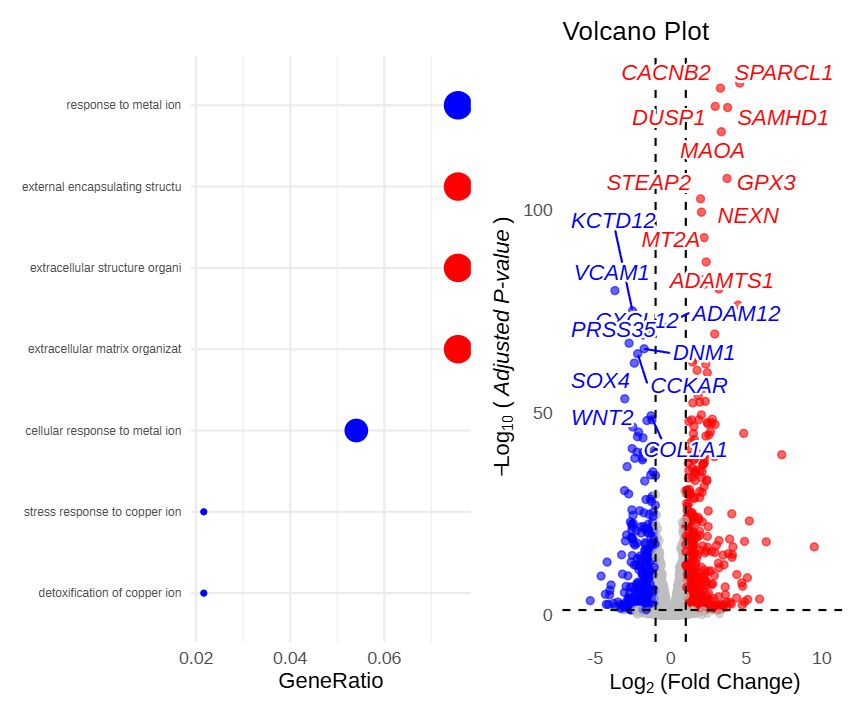
Figure 9 demonstrates the application of the pathway_volcano linkage function in multi-omics integrative analysis. After screening a large number of differentially expressed genes, enrichment analysis can be used to identify key pathways, and then the volcano plot can intuitively display the specific expression change direction and significance of genes within these pathways, facilitating rapid candidate biomarker screening.

References

1. Guangchuang Yu, et al. (2024). ivolcano: Interactive Volcano Plots. R package version 0.99.0.
2. ivolcano FigureYa wechat post