# Install packages
if (!requireNamespace("data.table", quietly = TRUE)) {
  install.packages("data.table")
}
if (!requireNamespace("jsonlite", quietly = TRUE)) {
  install.packages("jsonlite")
}
if (!requireNamespace("grafify", quietly = TRUE)) {
  install.packages("grafify")
}
if (!requireNamespace("ggplot2", quietly = TRUE)) {
  install.packages("ggplot2")
}

# Load packages
library(data.table)
library(jsonlite)
library(grafify)
library(ggplot2)Gradient Scatter
Note
Hiplot website
This page is the tutorial for source code version of the Hiplot Gradient Scatter plugin. You can also use the Hiplot website to achieve no code ploting. For more information please see the following link:
Two-dimensional spatial scatter to demonstrate multi-numerical variable relationships.
Setup
System Requirements: Cross-platform (Linux/MacOS/Windows)
Programming language: R
Dependent packages:
data.table;jsonlite;grafify;ggplot2
sessioninfo::session_info("attached")─ Session info ───────────────────────────────────────────────────────────────
setting value
version R version 4.6.0 (2026-04-24)
os Ubuntu 24.04.4 LTS
system x86_64, linux-gnu
ui X11
language (EN)
collate C.UTF-8
ctype C.UTF-8
tz UTC
date 2026-05-09
pandoc 3.1.3 @ /usr/bin/ (via rmarkdown)
quarto 1.9.37 @ /usr/local/bin/quarto
─ Packages ───────────────────────────────────────────────────────────────────
package * version date (UTC) lib source
data.table * 1.18.4 2026-05-06 [1] RSPM
ggplot2 * 4.0.3.9000 2026-05-04 [1] Github (tidyverse/ggplot2@6870419)
grafify * 5.1.0 2025-08-25 [1] RSPM
jsonlite * 2.0.0 2025-03-27 [1] RSPM
[1] /home/runner/work/_temp/Library
[2] /opt/R/4.6.0/lib/R/site-library
[3] /opt/R/4.6.0/lib/R/library
* ── Packages attached to the search path.
──────────────────────────────────────────────────────────────────────────────Data Preparation
# Load data
data <- data.table::fread(jsonlite::read_json("https://hiplot.cn/ui/basic/scatter-gradient/data.json")$exampleData[[1]]$textarea[[1]])
data <- as.data.frame(data)

# View data
head(data)
car mpg cyl disp hp drat wt qsec vs am gear carb
1 Mazda RX4 21.0 6 160 110 3.90 2.620 16.46 0 1 4 4
2 Mazda RX4 Wag 21.0 6 160 110 3.90 2.875 17.02 0 1 4 4
3 Datsun 710 22.8 4 108 93 3.85 2.320 18.61 1 1 4 1
4 Hornet 4 Drive 21.4 6 258 110 3.08 3.215 19.44 1 0 3 1
5 Hornet Sportabout 18.7 8 360 175 3.15 3.440 17.02 0 0 3 2
6 Valiant 18.1 6 225 105 2.76 3.460 20.22 1 0 3 1Visualization
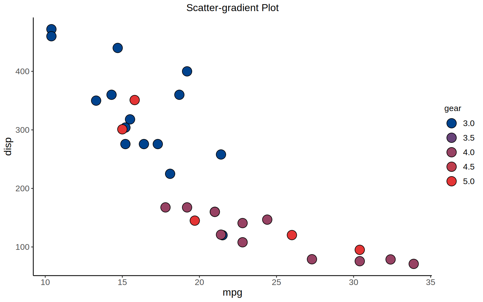
# Gradient Scatter
p <- ggplot(data, aes(x = mpg, y = disp)) +
  geom_point(aes(fill = gear), size = 5, alpha = 1, shape = 21, stroke = 0.5) +
  labs(fill = "gear", color = "gear") +
  theme_classic(base_size = 10) +
  theme(strip.background = element_blank()) +
  guides(x = guide_axis(angle = 0)) +
  scale_fill_gradient(low = "#00438E", high = "#E43535") +
  scale_color_gradient(low = "#00438E", high = "#E43535") +
  guides(fill = guide_legend(title = "gear"),
         size = guide_legend(title = "gear")) +
  ggtitle("Scatter-gradient Plot") +
  theme(text = element_text(family = "Arial"),
        plot.title = element_text(size = 12,hjust = 0.5),
        axis.title = element_text(size = 12),
        axis.text = element_text(size = 10),
        axis.text.x = element_text(angle = 0, hjust = 0.5,vjust = 1),
        legend.position = "right",
        legend.direction = "vertical",
        legend.title = element_text(size = 10),
        legend.text = element_text(size = 10))

p