Cell-Cell Communication Circle Plot

Authors

[Contributors] ShiXiang Wang.

Modified

2026-03-20

The Cell-Cell Communication Circle Plot (细胞-细胞通讯网络圈图) is a specialized visualization for depicting intercellular signaling interactions inferred from single-cell RNA sequencing (scRNA-seq) data. Using the CellChat R package, this plot presents a circular network where nodes represent cell populations (cell types or clusters) and directed edges indicate the strength and direction of ligand-receptor communication signals between them.

The arc width of each edge encodes communication probability, and the self-loops on each node represent autocrine signaling. Color coding maps each cell type to a distinct hue, and arrow directionality shows the sender-receiver relationship. This visualization is particularly powerful for discovering cross-talk between immune cells and tumor cells, identifying key signaling hubs in tissue microenvironments, and comparing communication networks across biological conditions.

Example

Cell-Cell Communication Circle Plot DEMO

Setup

System Requirements: Cross-platform (Linux/MacOS/Windows)
Programming Language: R
Dependencies: CellChat, ggplot2, circlize

# Install Bioconductor manager if needed
if (!requireNamespace("BiocManager", quietly = TRUE)) {
  install.packages("BiocManager")
}

# Install CRAN dependencies
if (!requireNamespace("ggplot2", quietly = TRUE)) install.packages("ggplot2")
if (!requireNamespace("circlize", quietly = TRUE)) install.packages("circlize")
if (!requireNamespace("igraph", quietly = TRUE)) install.packages("igraph")

# Install CellChat from GitHub (jinworks/CellChat is the current maintained fork)
if (!requireNamespace("CellChat", quietly = TRUE)) {
  if (!requireNamespace("remotes", quietly = TRUE)) install.packages("remotes")
  remotes::install_github("jinworks/CellChat")
}

# Load packages
library(CellChat)
library(ggplot2)
library(circlize)

sessioninfo::session_info("attached")

─ Session info ───────────────────────────────────────────────────────────────
 setting  value
 version  R version 4.5.3 (2026-03-11)
 os       Ubuntu 24.04.3 LTS
 system   x86_64, linux-gnu
 ui       X11
 language (EN)
 collate  C.UTF-8
 ctype    C.UTF-8
 tz       UTC
 date     2026-03-20
 pandoc   3.1.3 @ /usr/bin/ (via rmarkdown)
 quarto   1.8.27 @ /usr/local/bin/quarto

─ Packages ───────────────────────────────────────────────────────────────────
 package      * version    date (UTC) lib source
 Biobase      * 2.70.0     2025-10-29 [1] Bioconduc~
 BiocGenerics * 0.56.0     2025-10-29 [1] Bioconduc~
 CellChat     * 2.2.0.9001 2026-03-20 [1] Github (jinworks/CellChat@75253cd)
 circlize     * 0.4.17     2025-12-08 [1] RSPM
 dplyr        * 1.2.0      2026-02-03 [1] RSPM
 generics     * 0.1.4      2025-05-09 [1] RSPM
 ggplot2      * 4.0.2      2026-02-03 [1] RSPM
 igraph       * 2.2.2      2026-02-12 [1] RSPM

 [1] /home/runner/work/_temp/Library
 [2] /opt/R/4.5.3/lib/R/site-library
 [3] /opt/R/4.5.3/lib/R/library
 * ── Packages attached to the search path.

──────────────────────────────────────────────────────────────────────────────

Data Preparation

For this tutorial, we build a simulated CellChat-compatible communication matrix so the example is fully self-contained and runs without requiring an external dataset or model inference. The same visualizations work identically with a real CellChat object produced from your own scRNA-seq data.

# Simulate a communication count/weight matrix
# In real use, these come from cellchat@net$count and cellchat@net$weight

set.seed(42)
cell_types <- c("CD4 T", "CD8 T", "NK", "B cell", "Monocyte",
                "DC", "Fibroblast", "Epithelial", "Endothelial")
n <- length(cell_types)

net_count  <- matrix(sample(0:50, n * n, replace = TRUE), n, n,
                     dimnames = list(cell_types, cell_types))
net_weight <- matrix(runif(n * n, 0, 1), n, n,
                     dimnames = list(cell_types, cell_types))
diag(net_count)  <- 0  # remove self-communication
diag(net_weight) <- 0

# Group size (proportional to number of cells per type, simulated)
group_size <- sample(50:500, n, replace = TRUE)
names(group_size) <- cell_types

cat("Simulated", n, "cell types with", sum(net_count), "total interactions\n")

Simulated 9 cell types with 1875 total interactions

print(net_count)

            CD4 T CD8 T NK B cell Monocyte DC Fibroblast Epithelial Endothelial
CD4 T           0    23 46      4       29 44         48         37          41
CD8 T          36     0  2     19       42 27         25          9           8
NK              0    35  0     33       14  4         49         39          28
B cell         24    24 24      0       21  3          5          4          11
Monocyte        9    36 26     39        0 33          5         32          19
DC             35    45 35      2       35  0          1         48           8
Fibroblast     17    19 36     32        3 34          0         38          42
Epithelial     48    25 30     41       21 23         20          0          34
Endothelial    46    49 44     23       17 22          1         44           0

Build a CellChat Object from Your Own Data (Reference)

The following code is for reference only (eval: false). It shows how to build a CellChat object from a Seurat scRNA-seq object before running the visualizations below.

library(Seurat)
library(CellChat)

# 1. Extract normalised count matrix and metadata from a Seurat object
seurat_obj  <- readRDS("your_seurat_object.rds")
data_input  <- GetAssayData(seurat_obj, assay = "RNA", slot = "data")
meta        <- seurat_obj@meta.data

# 2. Create CellChat object
cellchat <- createCellChat(object = data_input, meta = meta, group.by = "cell_type")

# 3. Set ligand-receptor database
cellchat@DB <- CellChatDB.human  # or CellChatDB.mouse

# 4. Pre-process & infer communication
cellchat <- subsetData(cellchat)
cellchat <- identifyOverExpressedGenes(cellchat)
cellchat <- identifyOverExpressedInteractions(cellchat)
cellchat <- computeCommunProb(cellchat, type = "triMean")
cellchat <- filterCommunication(cellchat, min.cells = 10)
cellchat <- computeCommunProbPathway(cellchat)
cellchat <- aggregateNet(cellchat)
# Now cellchat@net$count and cellchat@net$weight are available for plotting

Visualization

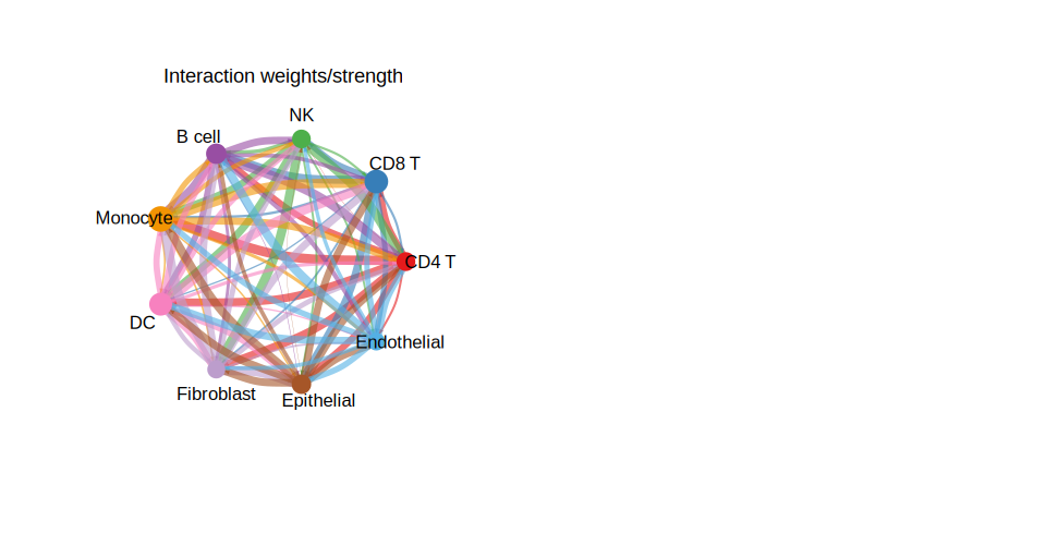
1. Circle Plot of Overall Cell-Cell Communication Network

The overall circle plot summarizes all inferred communication interactions. Each node represents a cell type; node size is proportional to the number of interactions it participates in. Arc width encodes communication strength.

par(mfrow = c(1, 2), xpd = TRUE)

# Panel A: Number of interactions
netVisual_circle(
  net_count,
  vertex.weight = group_size,
  weight.scale  = TRUE,
  label.edge    = FALSE,
  title.name    = "Number of interactions"
)

# Panel B: Interaction strength (weights)
netVisual_circle(
  net_weight,
  vertex.weight = group_size,
  weight.scale  = TRUE,
  label.edge    = FALSE,
  title.name    = "Interaction weights/strength"
)

par(mfrow = c(1, 1))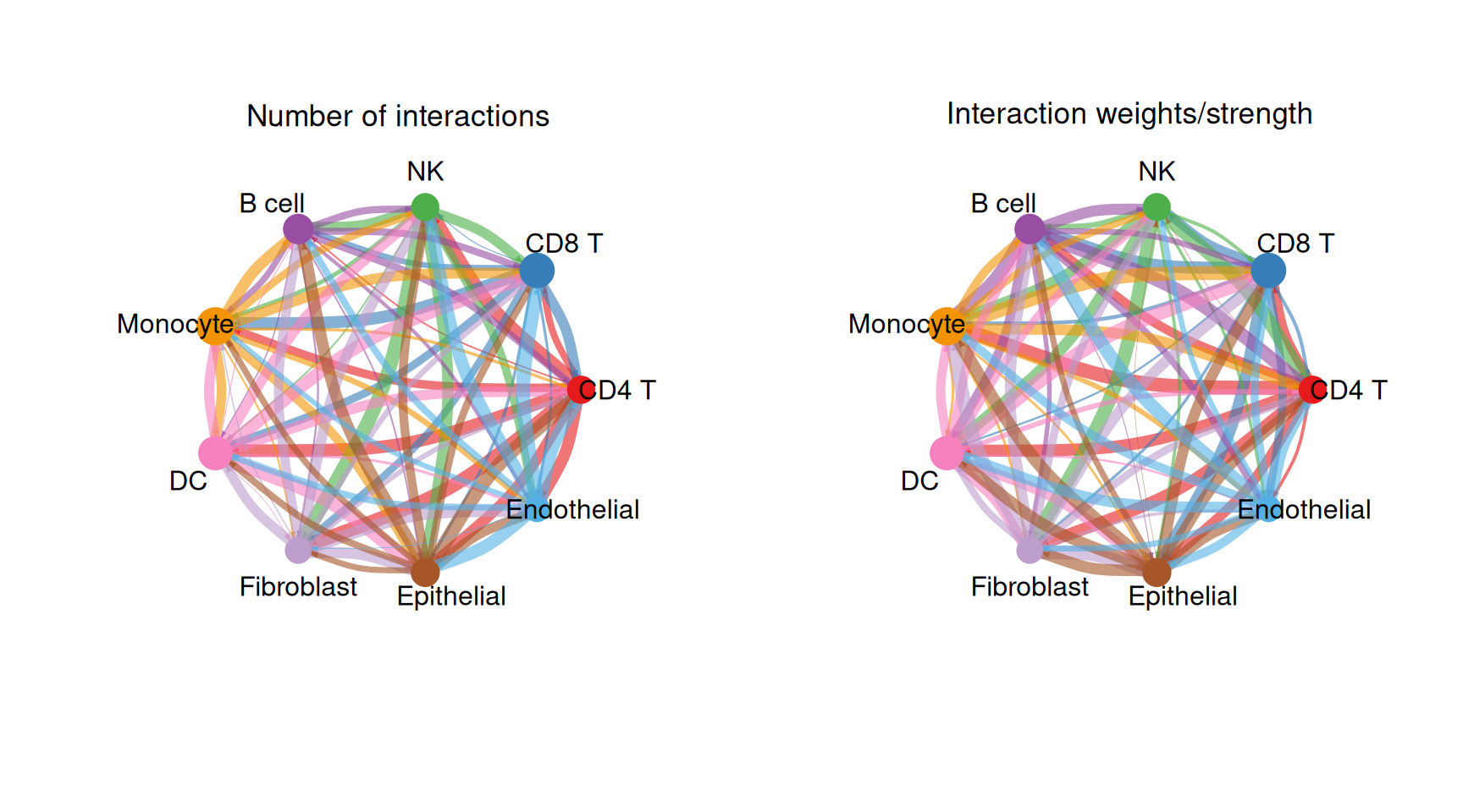

Figure 1: Overall Cell-Cell Communication Circle Plot

2. Circle Plot for Individual Cell Groups

To highlight the outgoing signals from each cell type separately, we subset the weight matrix row by row and produce one circle per cell type.

n_types <- nrow(net_weight)
n_cols  <- ceiling(sqrt(n_types))
n_rows  <- ceiling(n_types / n_cols)

par(mfrow = c(n_rows, n_cols), xpd = TRUE, mar = c(1, 1, 2, 1))

for (i in seq_len(n_types)) {
  mat_i          <- matrix(0, nrow = n_types, ncol = n_types,
                           dimnames = dimnames(net_weight))
  mat_i[i, ]    <- net_weight[i, ]   # outgoing signals from cell type i

  netVisual_circle(
    mat_i,
    vertex.weight   = group_size,
    weight.scale    = TRUE,
    edge.weight.max = max(net_weight),
    title.name      = rownames(net_weight)[i]
  )
}

par(mfrow = c(1, 1))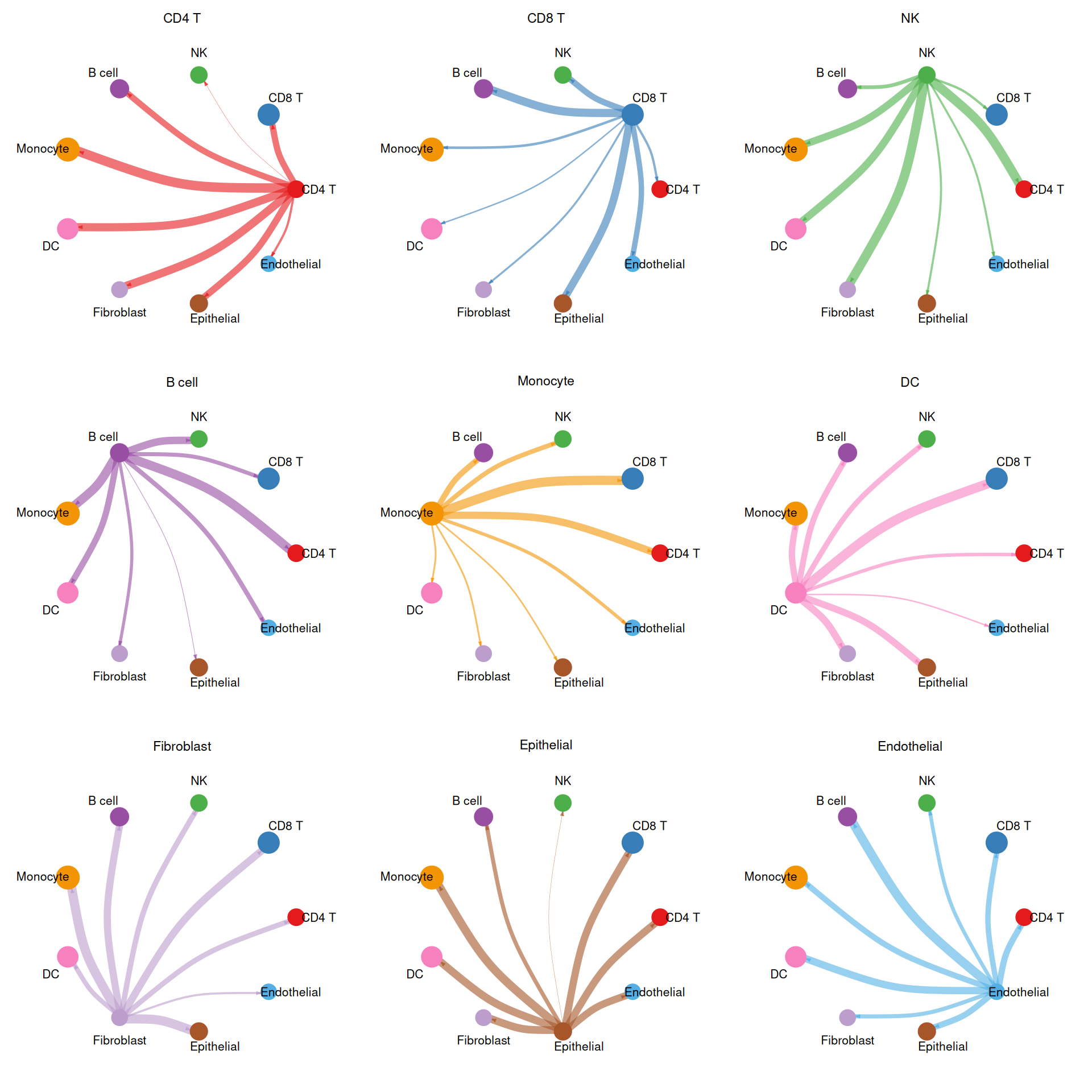

Figure 2: Per-Cell-Type Outgoing Communication Circle Plot

3. Chord Diagram

The chord diagram provides an alternative circular view using circlize, clearly showing bidirectional communication volumes between cell type pairs.

# Use circlize for a chord diagram of communication weights
chordDiagram(
  net_weight,
  transparency      = 0.4,
  annotationTrack   = "grid",
  preAllocateTracks = 1
)

circos.trackPlotRegion(
  track.index = 1,
  panel.fun   = function(x, y) {
    circos.text(
      CELL_META$xcenter,
      CELL_META$ylim[1] + 0.1,
      CELL_META$sector.index,
      facing     = "clockwise",
      niceFacing = TRUE,
      adj        = c(0, 0.5),
      cex        = 0.7
    )
  },
  bg.border = NA
)

title("Cell-Cell Communication (Chord Diagram)")
circos.clear()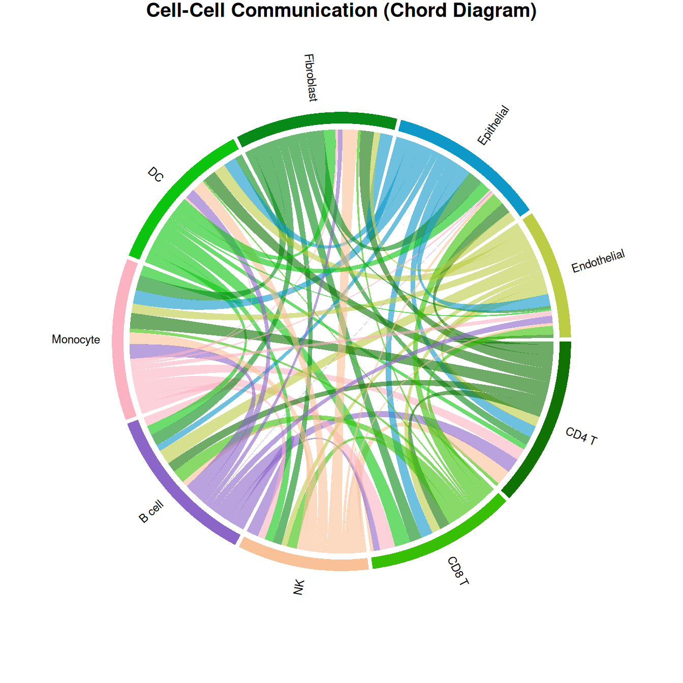

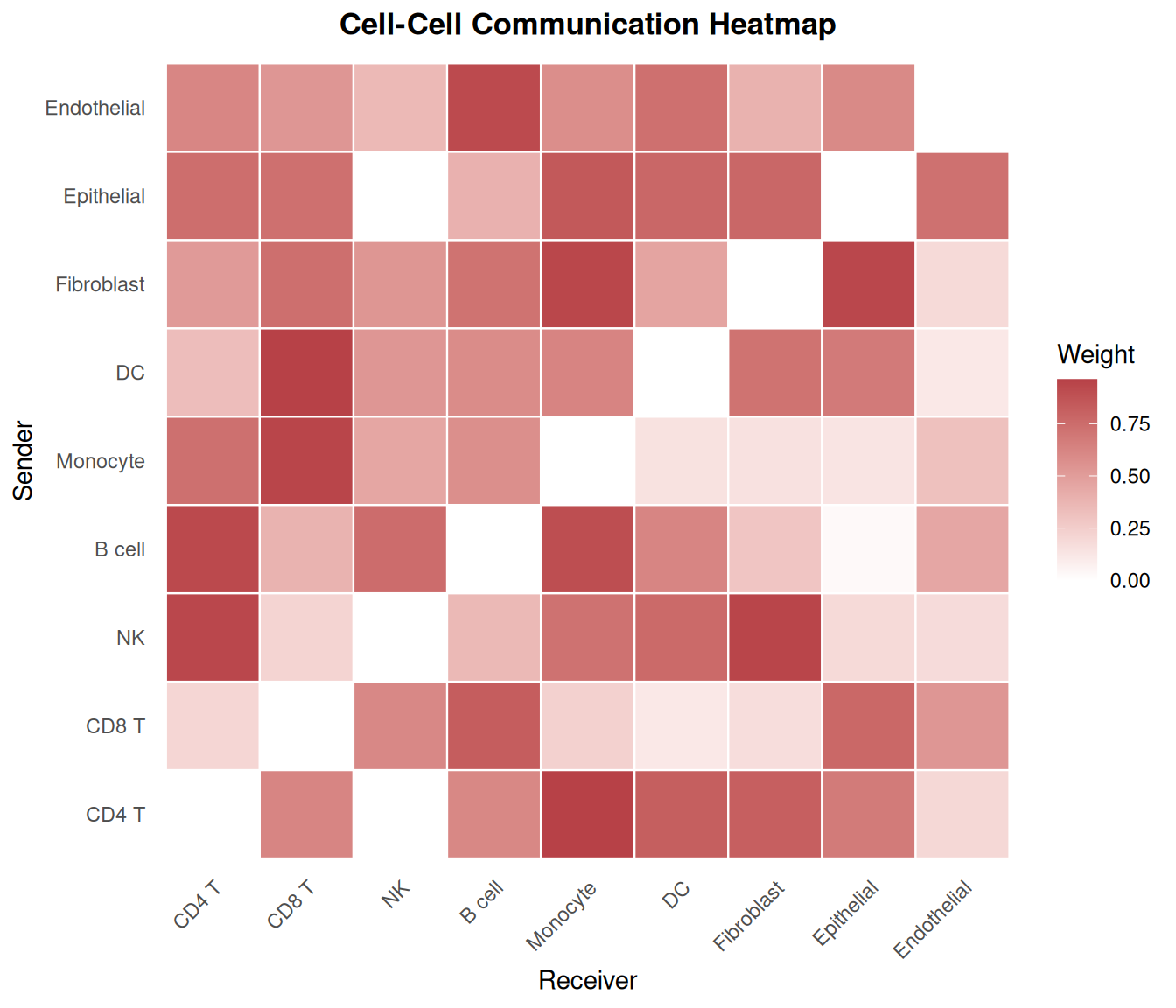
Figure 3: Cell-Cell Communication Chord Diagram

4. Communication Heatmap

A heatmap view allows rapid identification of dominant sender-receiver pairs and asymmetric communication patterns.

df_heat <- as.data.frame(as.table(net_weight))
colnames(df_heat) <- c("Sender", "Receiver", "Weight")

ggplot(df_heat, aes(x = Receiver, y = Sender, fill = Weight)) +
  geom_tile(color = "white", linewidth = 0.4) +
  scale_fill_gradient(low = "white", high = "#b74147", name = "Weight") +
  theme_minimal(base_size = 11) +
  theme(
    axis.text.x = element_text(angle = 45, hjust = 1),
    panel.grid  = element_blank(),
    plot.title  = element_text(size = 13, face = "bold", hjust = 0.5)
  ) +
  labs(
    title = "Cell-Cell Communication Heatmap",
    x = "Receiver", y = "Sender"
  )

Figure 4: Cell-Cell Communication Heatmap

References

[1] Jin S, Guerrero-Juarez CF, Zhang L, et al. Inference and analysis of cell-cell communication using CellChat. Nature Communications. 2021;12(1):1088. https://doi.org/10.1038/s41467-021-21246-9

[2] Jin S, et al. CellChat for systematic analysis of cell-cell communication from single-cell transcriptomics. Nature Protocols. 2024. https://doi.org/10.1038/s41596-024-01045-4

[3] CellChat GitHub: https://github.com/jinworks/CellChat