Manhattan & QQ Plot (Python)

🤖 AI Skill — Download the Bizard unified skill for your AI assistant ⬇️ Download Skill ZIP

🔌 MCP Server — Let AI agents (Claude Code, Cursor, …) query Bizard live: claude mcp add bizard -- npx @openbiox/bizard-mcp — or the free hosted instance (no install, faster from mainland China): claude mcp add --transport http bizard http://biotree.top:38123/bizard-mcp/mcp 📖 MCP Docs

📖 Cite Bizard — if Bizard helps your research, please cite: Li, K., Zheng, H., Huang, K., et al. (2026). Bizard: A Community-Driven Platform for Accelerating and Enhancing Biomedical Data Visualization. iMetaMed, e70038. 🔗 DOI / BibTeX

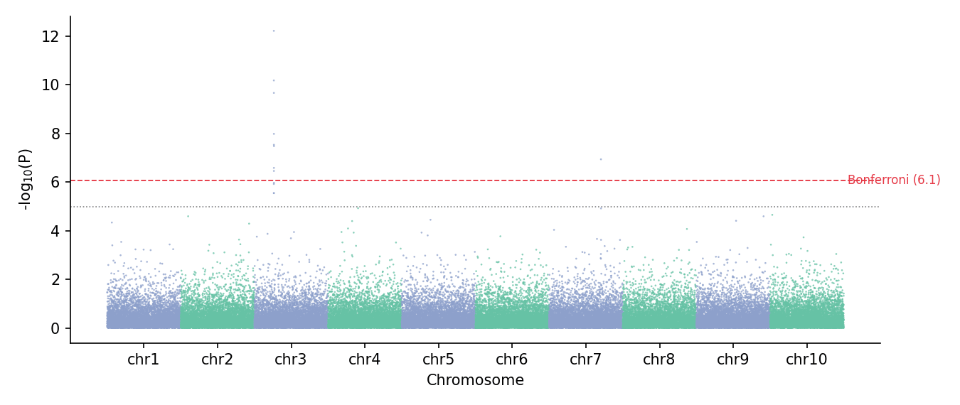
A Manhattan plot lines up every variant along the genome (x = chromosome position, y = −log10 p) so association peaks rise above the null skyline; its companion QQ plot compares the observed p-value distribution to the uniform expectation, with the genomic inflation factor λ summarizing confounding. Both are standard GWAS/QTL summaries assembled from scatter primitives in matplotlib.

Example

Setup

• System Requirements: Cross-platform (Linux/MacOS/Windows)
• Programming Language: Python
• Dependencies: matplotlib, pandas, numpy

import matplotlib.pyplot as plt
import pandas as pd
import numpy as np
from scipy.stats import chi2

Data Preparation

We simulate 60,000 SNPs over 10 chromosomes under the null (χ²₁ p-values) and inject one association peak on chromosome 3 plus a smaller one on chromosome 7.

np.random.seed(131)

chr_sizes = np.full(10, 6_000)
rows = []
snp_id = 0
for chr_id in range(1, 11):
    pos = np.sort(np.random.uniform(1, chr_sizes[chr_id - 1], 6_000))
    chisq = np.random.chisquare(1, 6_000)
    if chr_id == 3:
        chisq[1500:1512] = np.random.chisquare(30, 12)      # strong peak
    if chr_id == 7:
        chisq[4200:4206] = np.random.chisquare(14, 6)       # modest peak
    p = chi2.sf(chisq, 1)
    rows.append(pd.DataFrame({
        'CHR': chr_id, 'POS': pos, 'P': p,
        'SNP': [f'rs{snp_id + j}' for j in range(6_000)]}))
    snp_id += 6_000
gwas = pd.concat(rows, ignore_index=True)
gwas['minus_log_p'] = -np.log10(gwas.P)

# cumulative offset for genome-linear coordinates
offsets = {c: i * chr_sizes[i] for i, c in enumerate(range(1, 11))}
gwas['POS_cum'] = gwas.POS + gwas.CHR.map(offsets)
tick_df = gwas.groupby('CHR').POS_cum.agg(['min', 'max'])
chr_ticks = (tick_df['min'] + tick_df['max']) / 2
BONF = -np.log10(0.05 / len(gwas))
SUGG = -np.log10(1e-5)

Visualization

Classic Manhattan Plot

Alternating per-chromosome colours keep adjacent chromosomes separable; genome-wide and suggestive thresholds are drawn as horizontal guides.

fig, ax = plt.subplots(figsize=(9, 3.8))
chr_colors = np.where(gwas.CHR % 2 == 1, '#8da0cb', '#66c2a5')
ax.scatter(gwas.POS_cum, gwas.minus_log_p, s=1.6, c=chr_colors,
           alpha=0.75, linewidths=0, rasterized=True)
ax.axhline(BONF, color='#e63946', linewidth=0.9, linestyle='--')
ax.axhline(SUGG, color='0.5', linewidth=0.8, linestyle=':')
ax.text(len(gwas) * 1.005, BONF, f'Bonferroni ({BONF:.1f})',
        va='center', fontsize=8, color='#e63946')
ax.set_xticks(chr_ticks, [f'chr{c}' for c in chr_ticks.index])
ax.set_xlabel('Chromosome')
ax.set_ylabel('-log$_{10}$(P)')
ax.spines[['top', 'right']].set_visible(False)
plt.tight_layout()
plt.show()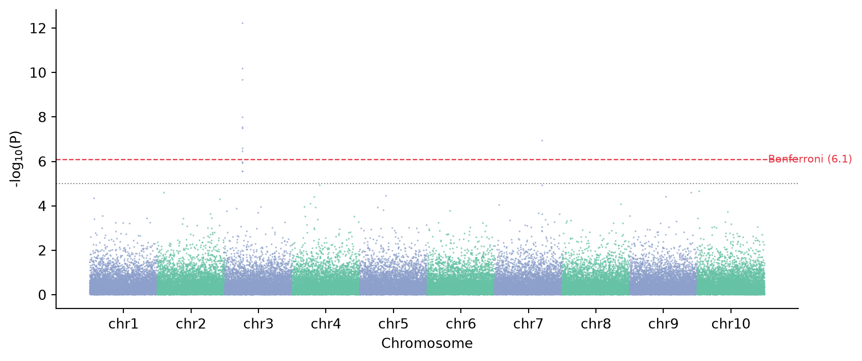

Figure 1: Manhattan plot of the simulated GWAS with Bonferroni and suggestive lines

QQ Plot with Inflation Factor

Ordered observed −log10 p against expected uniform quantiles; λ (median χ² ratio) quantifies inflation — λ ≈ 1 means no systematic confounding in the simulation.

obs = np.sort(gwas.minus_log_p)[::-1]
n = len(obs)
exp = -np.log10((np.arange(1, n + 1)) / (n + 1))
lam = np.median(chi2.ppf(1 - gwas.P, 1)) / chi2.median(1)

fig, ax = plt.subplots(figsize=(4.6, 4.6))
ax.scatter(exp, obs, s=3, color='#8da0cb', alpha=0.6, rasterized=True)
lim = max(exp.max(), obs.max()) * 1.05
ax.plot([0, lim], [0, lim], color='0.3', linewidth=0.9)
ax.set_xlabel(f'Expected -log$_{{10}}$(P)   (λ = {lam:.3f})')
ax.set_ylabel('Observed -log$_{10}$(P)')
ax.spines[['top', 'right']].set_visible(False)
plt.tight_layout()
plt.show()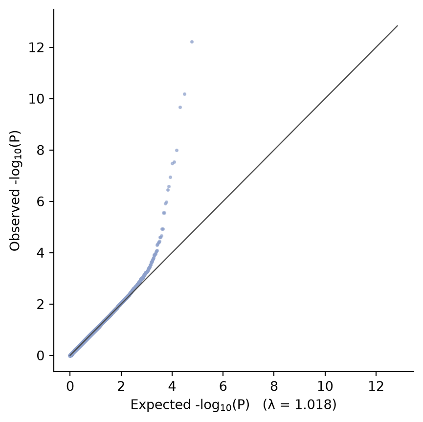

Figure 2: QQ plot of GWAS p-values with the genomic inflation factor

References

1. Turner, S., et al. (2011). Quality Control for Population Association Studies. PLoS Currents, 3, RRN1222.
2. Hunter, J. D. (2007). Matplotlib: A 2D graphics environment. Computing in Science & Engineering, 9(3), 90-95.