Box Plot (Python)

🤖 AI Skill — Download the Bizard unified skill for your AI assistant ⬇️ Download Skill ZIP

🔌 MCP Server — Let AI agents (Claude Code, Cursor, …) query Bizard live: claude mcp add bizard -- npx @openbiox/bizard-mcp — or the free hosted instance (no install, faster from mainland China): claude mcp add --transport http bizard http://biotree.top:38123/bizard-mcp/mcp 📖 MCP Docs

📖 Cite Bizard — if Bizard helps your research, please cite: Li, K., Zheng, H., Huang, K., et al. (2026). Bizard: A Community-Driven Platform for Accelerating and Enhancing Biomedical Data Visualization. iMetaMed, e70038. 🔗 DOI / BibTeX

A box plot summarizes the distribution of a numeric variable through its median, quartiles, and outliers. In biomedical research, box plots are the standard compact display for comparing biomarker levels across genotypes, batches, or treatment arms. Python’s seaborn builds directly on matplotlib to provide notched, grouped, and point-overlay variants suitable for publication figures.

Example

Setup

• System Requirements: Cross-platform (Linux/MacOS/Windows)
• Programming Language: Python
• Dependencies: matplotlib, seaborn, pandas, numpy

import matplotlib.pyplot as plt
import seaborn as sns
import pandas as pd
import numpy as np

Data Preparation

We simulate a serum biomarker assay across three genotypes (WT, HET, KO), with a sex factor for the grouped variant and enough replicates (n = 60 per genotype) for stable quartile estimates.

np.random.seed(7)

genotypes = ['WT', 'HET', 'KO']
n_per_genotype = 60
df = pd.DataFrame({
    'Genotype': np.repeat(genotypes, n_per_genotype),
    'Sex': np.tile(np.repeat(['Female', 'Male'], n_per_genotype // 2), 3),
    'Biomarker': np.concatenate([
        np.random.lognormal(1.2, 0.45, n_per_genotype),
        np.random.lognormal(1.55, 0.45, n_per_genotype),
        np.random.lognormal(1.95, 0.55, n_per_genotype),
    ])
})
# Inject a few extreme values in KO to demonstrate outlier display
df.loc[df.index[-3:], 'Biomarker'] *= 3.5

Visualization

Basic Box Plot

The box spans the interquartile range (IQR), the line marks the median, and whiskers extend to 1.5 × IQR; points beyond are drawn as fliers (outliers).

plt.figure(figsize=(5.5, 4.2))
ax = sns.boxplot(data=df, x='Genotype', y='Biomarker',
                 color='#8da0cb', width=0.5, linewidth=1.0,
                 fliersize=3, flierprops=dict(markerfacecolor='0.4'))
ax.set_xlabel('Genotype')
ax.set_ylabel('Biomarker level (ng/mL)')
ax.spines[['top', 'right']].set_visible(False)
plt.tight_layout()
plt.show()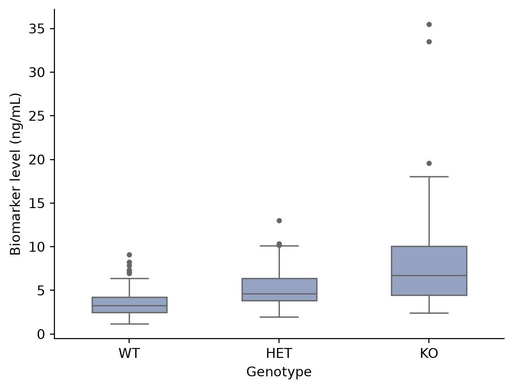

Figure 1: Box plot of serum biomarker across genotypes

Box Plot with Jittered Points

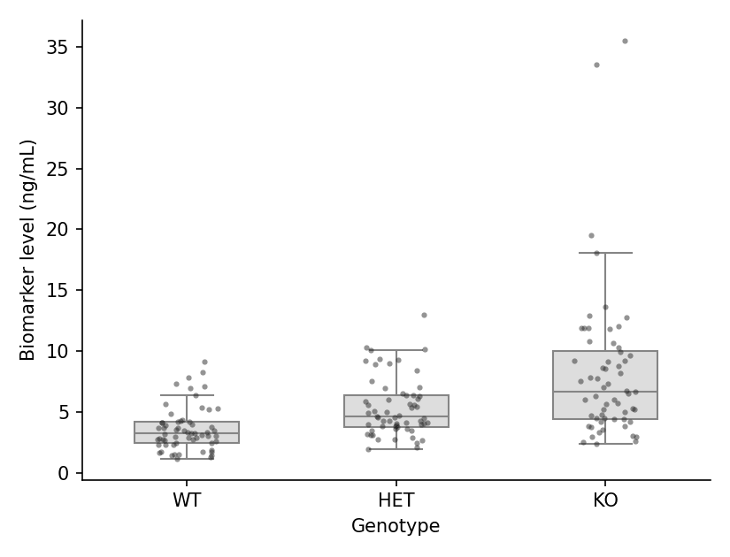
Because a box hides the raw data, overlaying the individual observations is the publication-recommended style: set showfliers=False and add a stripplot layer.

plt.figure(figsize=(5.5, 4.2))
ax = sns.boxplot(data=df, x='Genotype', y='Biomarker',
                 color='#dddddd', width=0.5, linewidth=1.0,
                 showfliers=False)
sns.stripplot(data=df, x='Genotype', y='Biomarker',
              color='#2b2b2b', size=3, alpha=0.5, jitter=0.15, ax=ax)
ax.set_xlabel('Genotype')
ax.set_ylabel('Biomarker level (ng/mL)')
ax.spines[['top', 'right']].set_visible(False)
plt.tight_layout()
plt.show()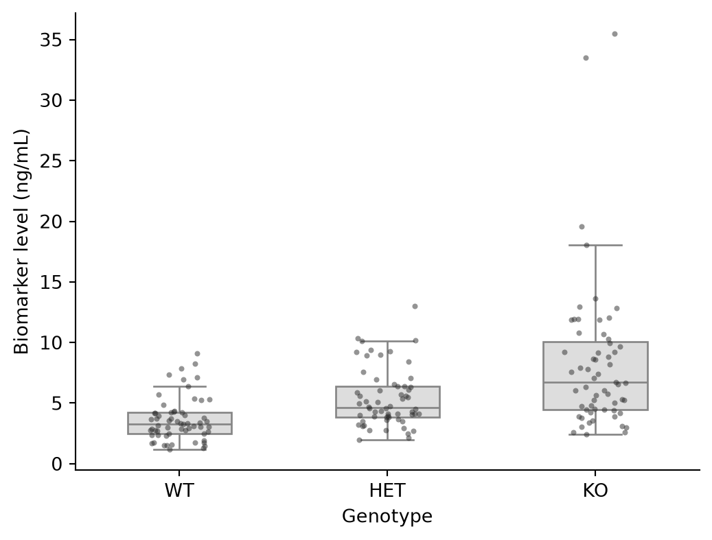

Figure 2: Box plot overlaid with individual data points

Grouped Box Plot

A second factor is mapped to hue, producing paired boxes within each category — the typical pre/post or two-cohort comparison.

plt.figure(figsize=(6.5, 4.2))
ax = sns.boxplot(data=df, x='Genotype', y='Biomarker', hue='Sex',
                 palette={'Female': '#e78ac3', 'Male': '#8da0cb'},
                 width=0.6, linewidth=1.0, fliersize=2.5)
ax.set_xlabel('Genotype')
ax.set_ylabel('Biomarker level (ng/mL)')
ax.legend(frameon=False, title=None)
ax.spines[['top', 'right']].set_visible(False)
plt.tight_layout()
plt.show()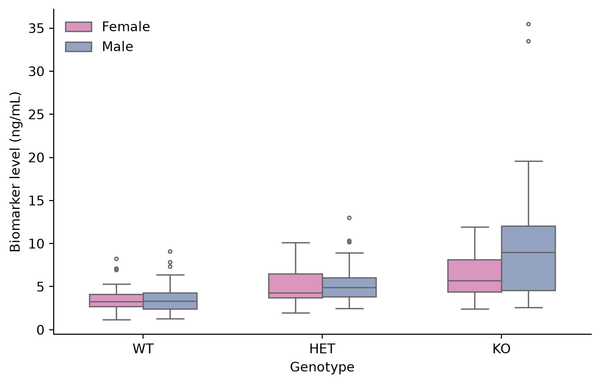

Figure 3: Grouped box plot with a sex factor

Notched Box Plot

The notch approximates a 95% confidence interval around the median; non-overlapping notches between two boxes are informal evidence of different medians.

plt.figure(figsize=(5.5, 4.2))
ax = sns.boxplot(data=df, x='Genotype', y='Biomarker',
                 color='#a6d854', width=0.5, linewidth=1.0,
                 notch=True, fliersize=3)
ax.set_xlabel('Genotype')
ax.set_ylabel('Biomarker level (ng/mL)')
ax.spines[['top', 'right']].set_visible(False)
plt.tight_layout()
plt.show()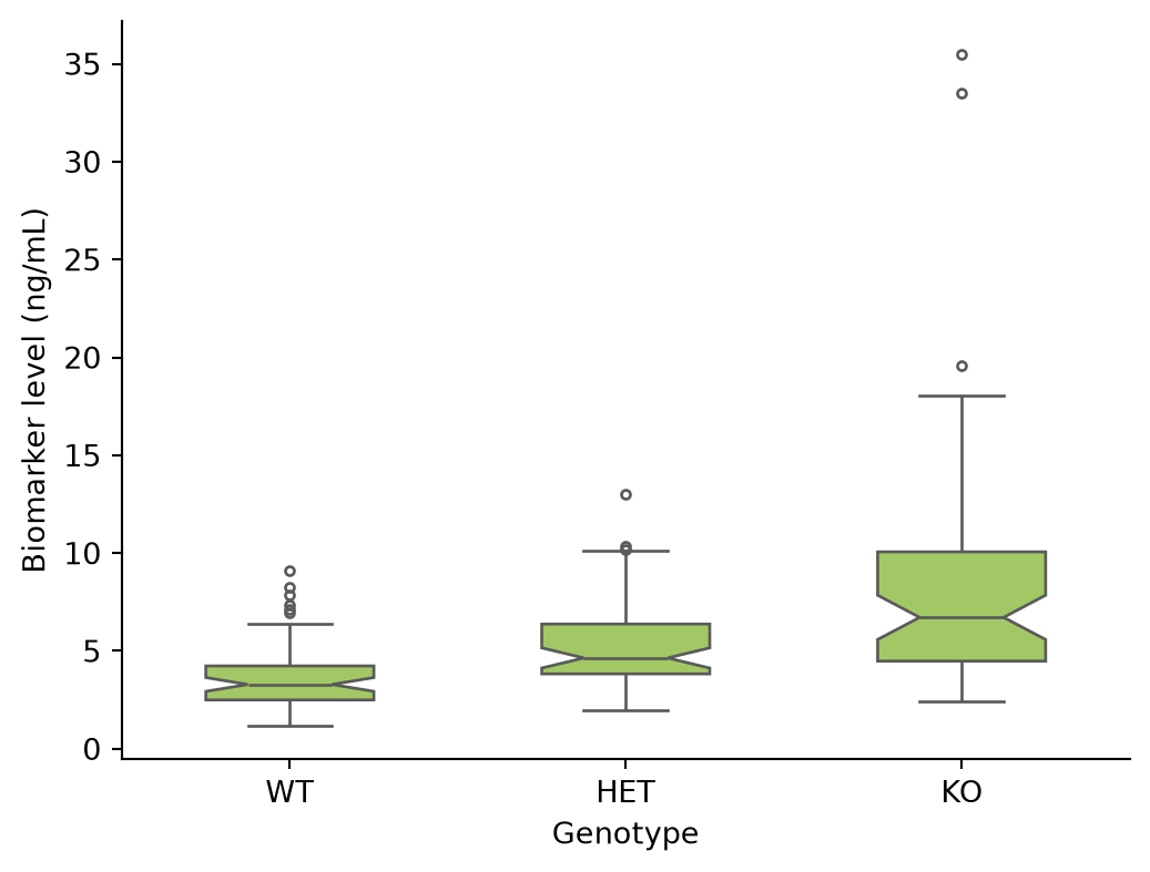

Figure 4: Notched box plot; notches approximate the median 95% CI

References

1. Hunter, J. D. (2007). Matplotlib: A 2D graphics environment. Computing in Science & Engineering, 9(3), 90-95.
2. Waskom, M. L. (2021). seaborn: statistical data visualization. Journal of Open Source Software, 6(60), 3021.
3. Spitzer, M., Wildenhain, J., Rappsilber, J., & Tyers, M. (2014). BoxPlotR: a web tool for generation of box plots. Nature Methods, 11(2), 121-122.