Immune-Related LncRNA Identification

Author

[Editor] ZCode (GLM) — AI-generated, independently AI-reviewed;

Modified

2026-11-05

🤖 AI Skill — Download the Bizard unified skill for your AI assistant ⬇️ Download Skill ZIP

🔌 MCP Server — Let AI agents (Claude Code, Cursor, …) query Bizard live: claude mcp add bizard -- npx @openbiox/bizard-mcp — or the free hosted instance (no install, faster from mainland China): claude mcp add --transport http bizard http://biotree.top:38123/bizard-mcp/mcp 📖 MCP Docs

📖 Cite Bizard — if Bizard helps your research, please cite: Li, K., Zheng, H., Huang, K., et al. (2026). Bizard: A Community-Driven Platform for Accelerating and Enhancing Biomedical Data Visualization. iMetaMed, e70038. 🔗 DOI / BibTeX

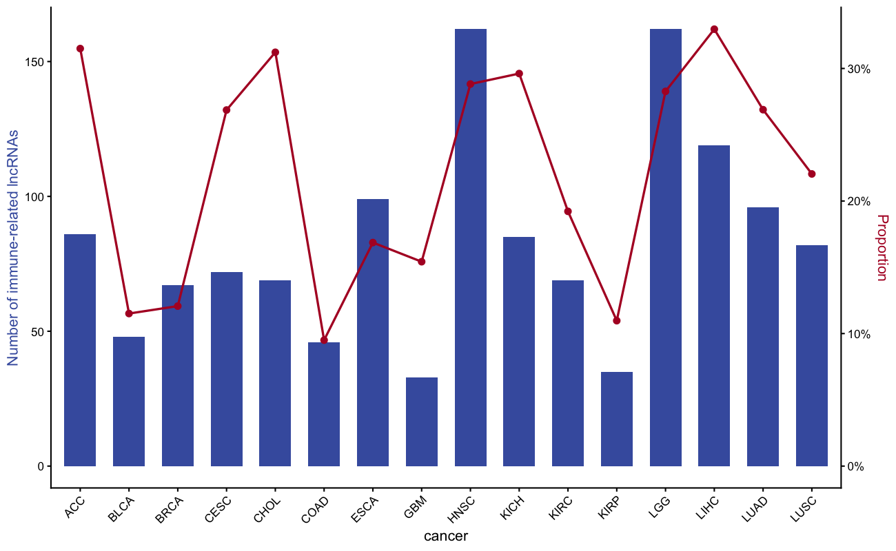
Identifying immune-related lncRNAs uses partial correlation between lncRNA expression and immune gene sets, followed by GSEA [1]. The canonical figure is a dual-axis bar + line chart: bars show the number of immune-related lncRNAs per cancer type (top y-axis) while a line shows the proportion (bottom y-axis).

Example

Setup

System Requirements: Cross-platform (Linux/MacOS/Windows)
Programming Language: R
Dependent packages: ggplot2; dplyr; scales

if (!requireNamespace("ggplot2", quietly = TRUE)) install.packages("ggplot2")
if (!requireNamespace("dplyr", quietly = TRUE)) install.packages("dplyr")
if (!requireNamespace("scales", quietly = TRUE)) install.packages("scales")

library(ggplot2)
library(dplyr)
library(scales)

sessioninfo::session_info("attached")

─ Session info ───────────────────────────────────────────────────────────────
 setting  value
 version  R version 4.6.2 (2026-10-29)
 os       Ubuntu 26.04.1 LTS
 system   x86_64, linux-gnu
 ui       X11
 language (EN)
 collate  C.UTF-8
 ctype    C.UTF-8
 tz       UTC
 date     2026-11-05
 pandoc   3.7.0.2 @ /usr/bin/ (via rmarkdown)
 quarto   1.11.9 @ /usr/local/bin/quarto

─ Packages ───────────────────────────────────────────────────────────────────
 ! package * version    date (UTC) lib source
 P dplyr   * 1.2.1      2026-04-03 [?] RSPM
 P ggplot2 * 4.0.3.9000 2026-11-03 [?] Github (tidyverse/ggplot2@b638d65)
 P scales  * 1.4.0      2025-04-24 [?] RSPM

 [1] /home/runner/.cache/R/renv/library/Bizard-5140bdc6/linux-ubuntu-resolute/R-4.6/x86_64-pc-linux-gnu
 [2] /home/runner/work/_temp/Library
 [3] /opt/R/4.6.2/lib/R/library

 * ── Packages attached to the search path.
 P ── Loaded and on-disk path mismatch.

──────────────────────────────────────────────────────────────────────────────

Data Preparation

With real data, immune-related lncRNAs are identified per cancer type via the ImmuLncRNA algorithm (partial correlation + GSEA). We simulate the per-cancer-type summary output: the number of immune-related lncRNAs and the total lncRNA count, from which the proportion is derived.

set.seed(1801)
cancers <- c("ACC", "BLCA", "BRCA", "CESC", "CHOL", "COAD", "ESCA", "GBM",
             "HNSC", "KICH", "KIRC", "KIRP", "LGG", "LIHC", "LUAD", "LUSC")
n_lnc_total <- sample(200:600, length(cancers))
n_immune    <- round(n_lnc_total * runif(length(cancers), 0.08, 0.35))

df <- data.frame(cancer = cancers,
                 total = n_lnc_total,
                 immune = n_immune) |>
  mutate(prop = immune / total)
head(df)

  cancer total immune       prop
1    ACC   273     86 0.31501832
2   BLCA   417     48 0.11510791
3   BRCA   555     67 0.12072072
4   CESC   268     72 0.26865672
5   CHOL   221     69 0.31221719
6   COAD   484     46 0.09504132

Visualization

1. Dual-Axis Bar + Line Chart

max_count <- max(df$immune)
max_prop  <- max(df$prop)

ggplot(df, aes(cancer, immune)) +
  geom_col(fill = "#445EAD", width = 0.65) +
  geom_line(aes(cancer, prop * max_count / max_prop, group = 1),
            colour = "#B2182B", linewidth = 0.8) +
  geom_point(aes(cancer, prop * max_count / max_prop),
             colour = "#B2182B", size = 2) +
  scale_y_continuous(
    name = "Number of immune-related lncRNAs",
    sec.axis = sec_axis(~ . * max_prop / max_count,
                        name = "Proportion",
                        labels = percent)) +
    labs(title = "Immune-related lncRNAs across cancer types") +
  theme_classic(base_size = 11) +
  theme(axis.text.x = element_text(angle = 45, hjust = 1),
        axis.title.y.left = element_text(colour = "#445EAD"),
        axis.title.y.right = element_text(colour = "#B2182B"))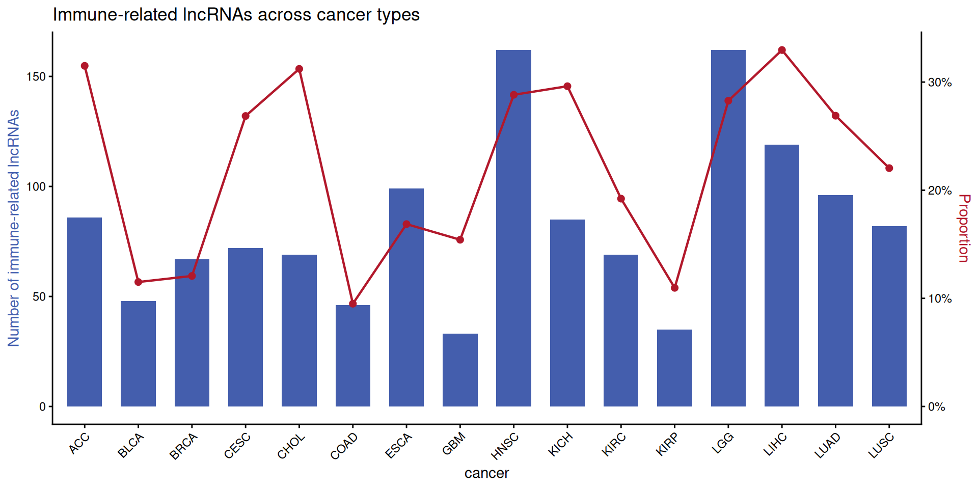

Figure 1: Dual-axis chart: bars = number of immune-related lncRNAs (left), line = proportion of immune-related lncRNAs (right), per cancer type.

Tip

Practice tips

The scaling factor max_count / max_prop aligns the two y-axes so the line sits within the bar range; adjust to avoid visual clutter.
Colour-code the two y-axis titles to match the bar and line colours — readers instinctively match axis title colour to the corresponding layer.
The reference workflow uses the ImmuLncRNA package (partial correlation + GSEA); the dual-axis chart is the summary visualisation of its output.

Application

Immune-related lncRNA identification is the first step in immune-lncRNA biomarker studies; the dual-axis chart compares yield across cancer types.

Reference

[1] Xiaofan Lu, et al. FigureYa: A Standardized Visualization Framework for Enhancing Biomedical Data Interpretation and Research Efficiency. iMetaMed. 2025. doi:10.1002/imm3.70005