Wordcloud

A word cloud is a visual representation of text words, which allows you to clearly see the keywords (high-frequency words) in a large amount of text data.

Example

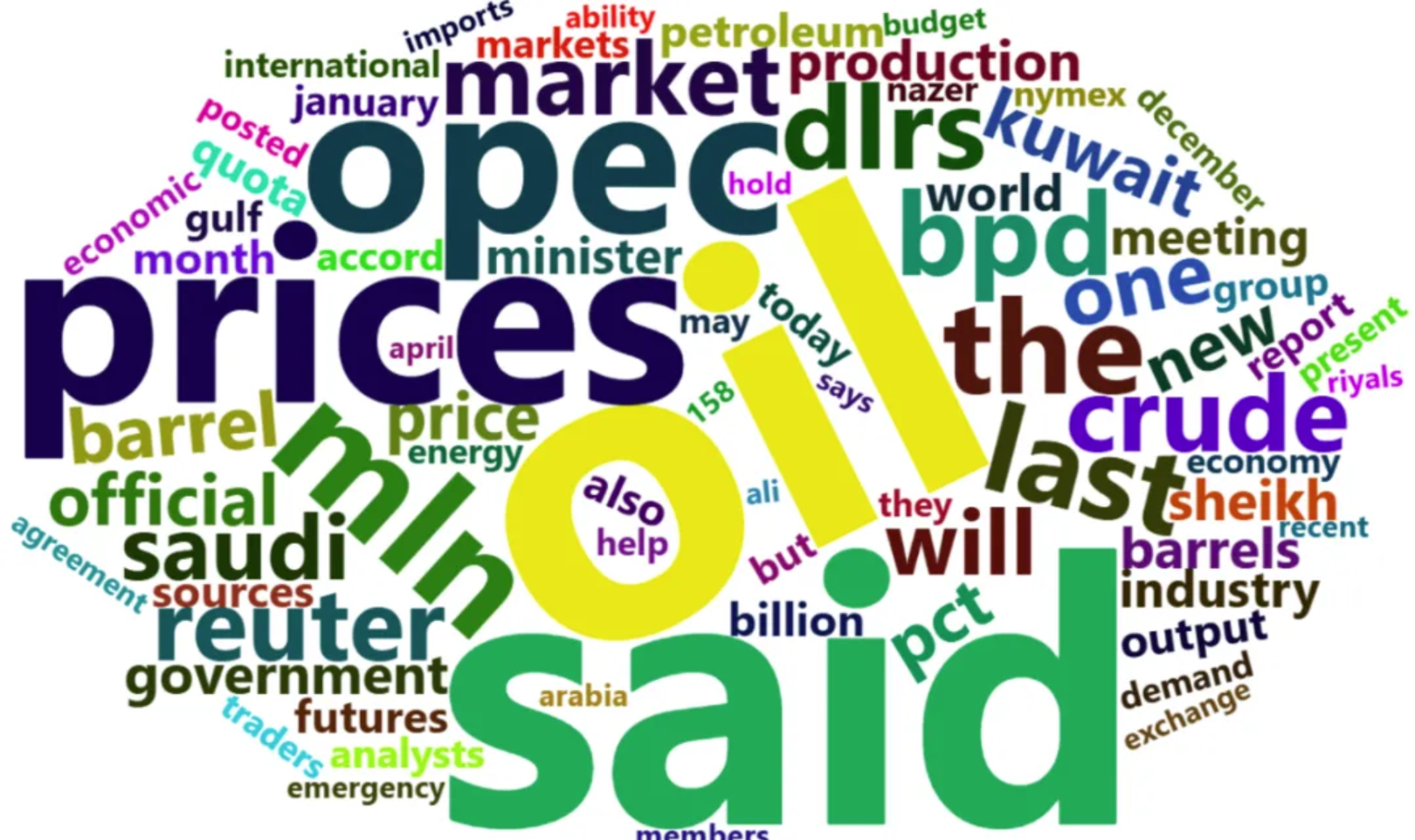
The image above shows a word cloud for an English text. The more frequent a word is, the larger it is. We can clearly identify the most frequent words from the word cloud, which are also the key words in the text. Displaying a large text as a word cloud allows us to understand the main content of the text in a shorter time.

Setup

• System Requirements: Cross-platform (Linux/MacOS/Windows)

• Programming Language: R

• Dependencies: wordcloud2, jiebaRD, jiebaR, dplyr, tidyverse, htmlwidgets, webshot2

# Install packages
if (!requireNamespace("wordcloud2", quietly = TRUE)) {
  install.packages("wordcloud2")
}
if (!requireNamespace("jiebaRD", quietly = TRUE)) {
  install.packages("https://cran.r-project.org/src/contrib/Archive/jiebaRD/jiebaRD_0.1.tar.gz")
}
if (!requireNamespace("jiebaR", quietly = TRUE)) {
  install.packages("https://cran.r-project.org/src/contrib/Archive/jiebaR/jiebaR_0.11.1.tar.gz")
}
if (!requireNamespace("dplyr", quietly = TRUE)) {
  install.packages("dplyr")
}
if (!requireNamespace("tidyverse", quietly = TRUE)) {
  install.packages("tidyverse")
}
if (!requireNamespace("htmlwidgets", quietly = TRUE)) {
  install.packages("htmlwidgets")
}
if (!requireNamespace("webshot2", quietly = TRUE)) {
  install.packages("webshot2")
}

# Load packages
library(wordcloud2)
library(jiebaR)    # Breaking Chinese text into words
library(dplyr)
library(tidyverse)
library(htmlwidgets)
library(webshot2)

Data Preparation

The Chinese texts used were 25 Chinese abstracts on immunotherapy for lung cancer retrieved from CNKI; the English texts used were the demoFreq dataset provided by R and 24 English abstracts on immunotherapy for lung cancer retrieved from PubMed.

# 1.Chinese abstract text
words <- read.csv("https://bizard-1301043367.cos.ap-guangzhou.myqcloud.com/words.txt",header = FALSE,sep="\n")
words <- as.character(words)

head_words <- substr(words, start = 1, stop = 20)

head_words

[1] "肺癌可分为非小细胞肺癌(NSCLC)和小"

# 2.demoFreq dataset
data <- demoFreq

head(data)

         word freq
oil       oil   85
said     said   73
prices prices   48
opec     opec   42
mln       mln   31
the       the   26

# 3.English abstract text
words_english <- read.csv("https://bizard-1301043367.cos.ap-guangzhou.myqcloud.com/words_english.txt",header = FALSE,sep="\n")

words_english <- as.character(words_english)

head_words_english <- substr(words_english, start = 1, stop = 20)

head_words_english

[1] "Persistent inflammat"

Convert text into phrases/words

Tip

Note: You can directly use the sample data demoFreq, so you don’t need to understand the text preprocessing process. The following mainly uses Chinese text for drawing.

Chinese text

# Use the jiebaR package to split the text into phrases
words_seg <- words %>%
  segment(worker()) %>%                    # Split text into words
  tibble(word = .) %>%  
  filter(nchar(word) > 1) %>%              # Remove single-word phrases
  count(word, sort = TRUE) %>%             # Statistical word frequency
  filter(!str_detect(word, "[0-9]+")) %>%  # Remove numbers
  slice_max(n, n = 50)                     # Select words with high frequency

head(words_seg)

# A tibble: 6 × 2
  word         n
  <chr>    <int>
1 患者       153
2 治疗        79
3 免疫治疗    64
4 NSCLC       55
5 细胞        55
6 肺癌        54

English text

# Split directly into single words
words_english %>%
 str_replace_all(",", " ") %>%         # Replace punctuation marks with spaces
 str_replace_all("\\.", " ") %>%
 str_replace_all("\\(", " ") %>%
 str_replace_all("\\)", " ") %>%
 str_split(" ", simplify = TRUE) %>%  # Split text into words
 .[nchar(.) > 1] %>%                  # Remove words of length 1 or 0
 tibble(word = .) %>%
 filter(!grepl("[0-9]+", word)) %>%   # Remove numbers
 table() %>%
 as.data.frame() %>%
 arrange(desc(Freq)) %>%
 slice(1:60) -> words_english_sep     # Select the top 60 words

# Remove meaningless words based on the word list
words_english_sep1 <- words_english_sep[c(-1, -2, -3, -4, -5, -6, -7, -14, -20, -22, -23, -24, -26, -27, -29, -30, -31, -33, -34, -35, -36, -44, -46, -53, -55),]

head(words_english_sep1)

            word Freq
8       patients   56
9  immunotherapy   51
10        cancer   46
11         NSCLC   46
12          lung   44
13          cell   40

The figure shows the words with higher frequency and their frequency after being split into words.

Visualization

1. Basic Plotting

# Basic Plotting
BasicPlot <- wordcloud2(data = words_seg, size = 1)
BasicPlot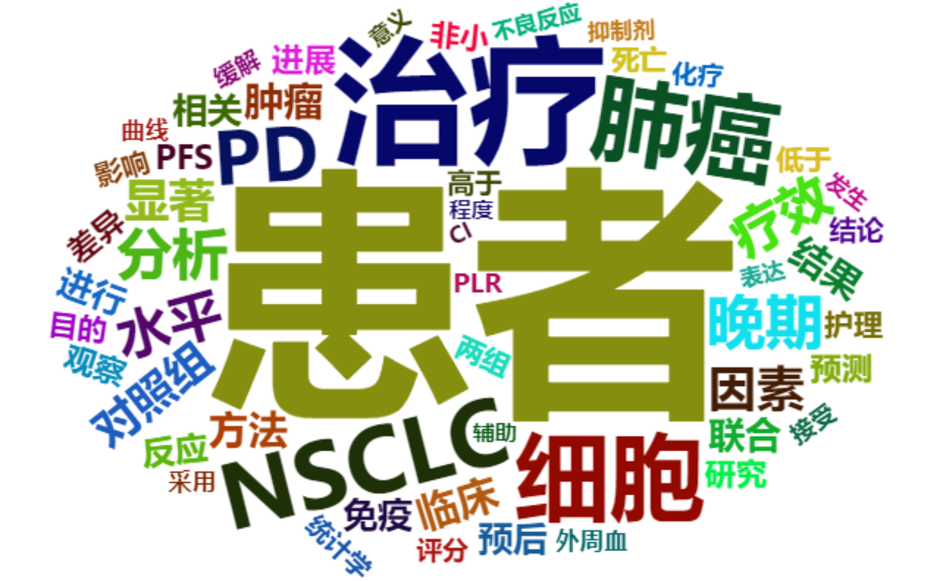

Figure 1: Basic Plotting

This figure is a basic word cloud diagram, which can be drawn by using the wordcloud2 function and word frequency data.

2. Set Color

color parameter

# (1) Set text color
Setcolors <- wordcloud2(data = words_seg, size = 1, color = "random-dark")
Setcolors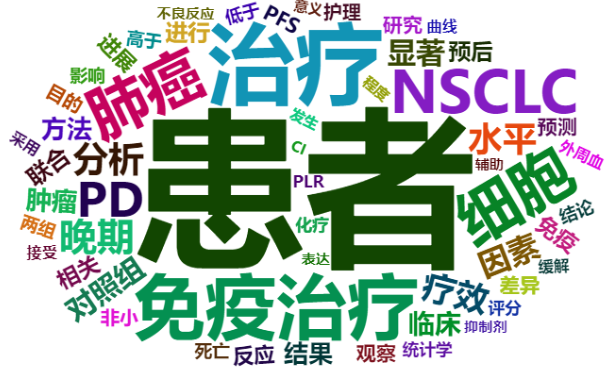

Figure 2: color parameter

This image uses the color parameter to set the word color to a random dark tone.

Tip

Key parameter: color

The color of the text. The options are “random-dark”, “random-light”, or you can use a vector to define a custom color.

Custom colors

# (2) Vector custom color
CustomizeColors <- wordcloud2(
  data = words_seg, size = 1, 
  color = rep_len(c("green", "blue"),nrow(words_seg)))
CustomizeColors

Figure 3: Custom colors

In this figure, the rep_len() function is used to repeat two colors to form a vector for the definition of word color.

Background Color

# (3) Set the background color
BackgroundColor <- wordcloud2(data = words_seg, size = 1, color = "random-light",
                              backgroundColor = "black")
BackgroundColor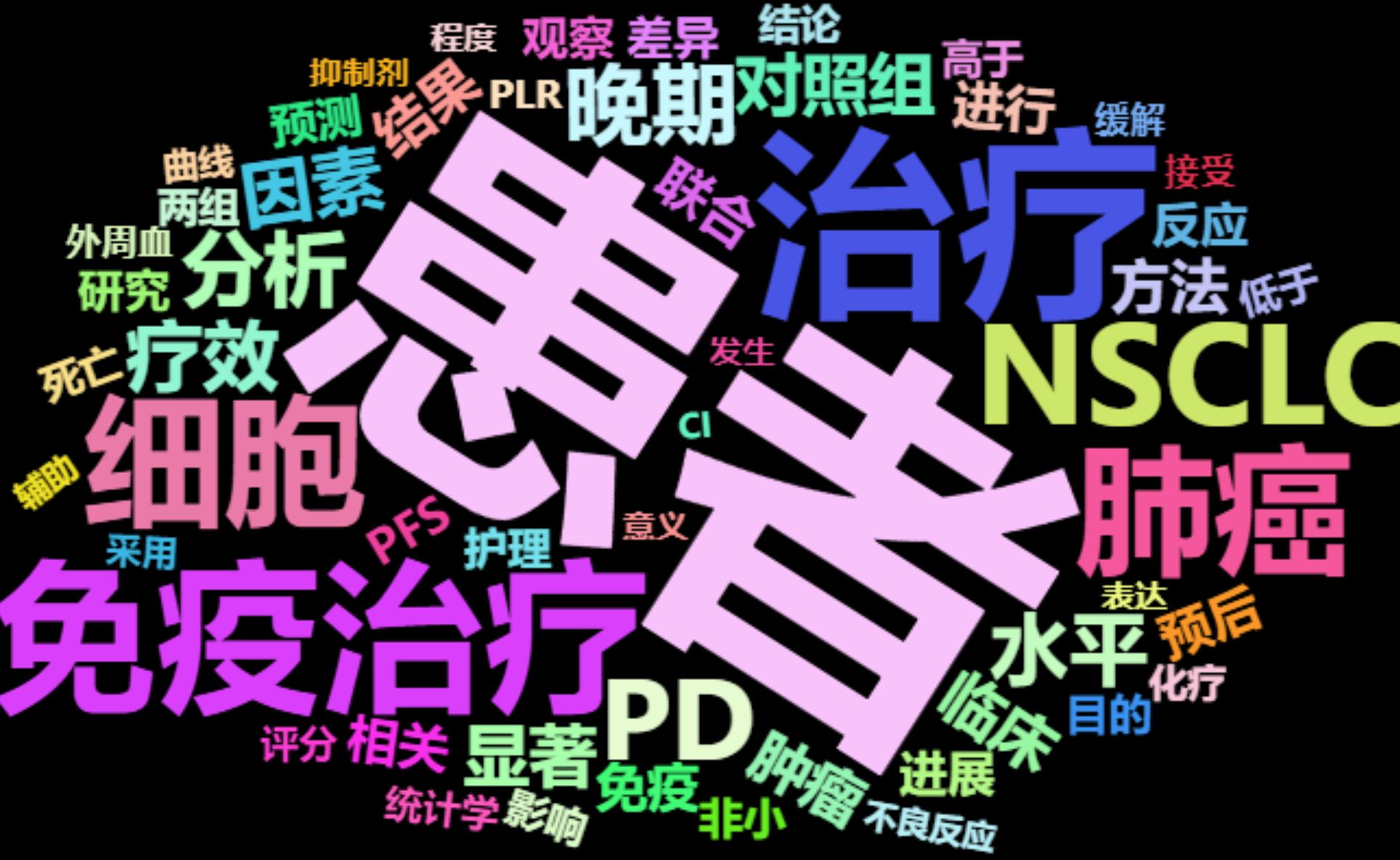

Figure 4: Background Color

This figure sets the color of the word cloud to the background color through backgroundColor="black" in the code.

3. Set shape

# Set as star
SetShape <- wordcloud2(data = words_seg, size = 0.5, shape = "star")
SetShape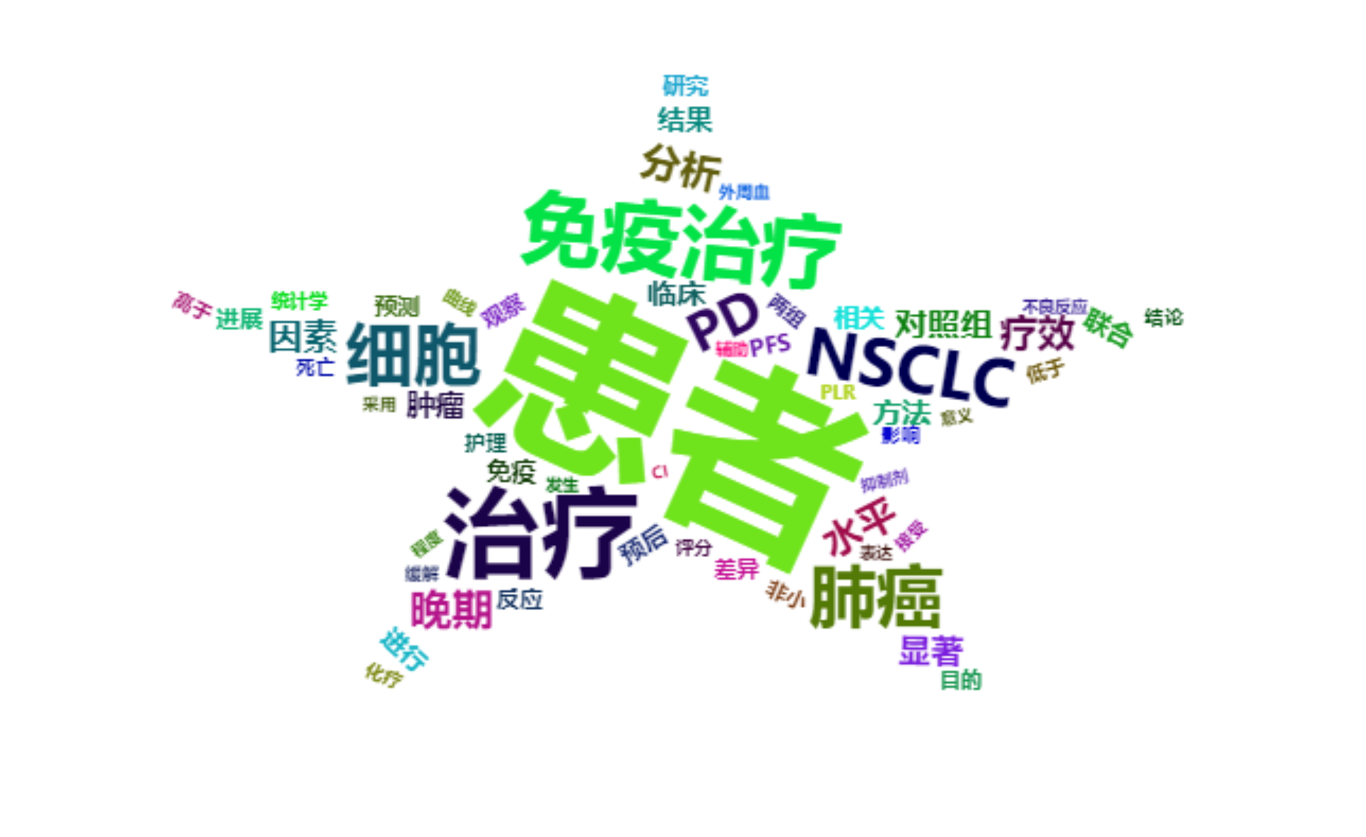

Figure 5: Set shape

This figure sets the shape of the word cloud to a star by shape = 'star' in the code. In addition to the star shape, there are many other shapes that can be used to make the word cloud drawing more personalized.

Tip

Key parameter: shape

The shape of the word cloud. The options are ‘circle’ (default, original shape), ‘cardioid’ (heart shape), ‘diamond’ (diamond shape), ‘triangle-forward’ (triangle-forward), ‘triangle’ (triangle), ‘pentagon’ (pentagon), ‘star’ (star shape).

4. Word Cloud Rotation

Fixed rotation

# (1) Set a certain rotation angle (the maximum and minimum angles are set to the same, and the rotation ratio is 1)
SpecificRotation <- wordcloud2(data = words_seg, size = 1, minRotation = -pi / 6,
                               maxRotation = -pi / 6, rotateRatio = 1)
SpecificRotation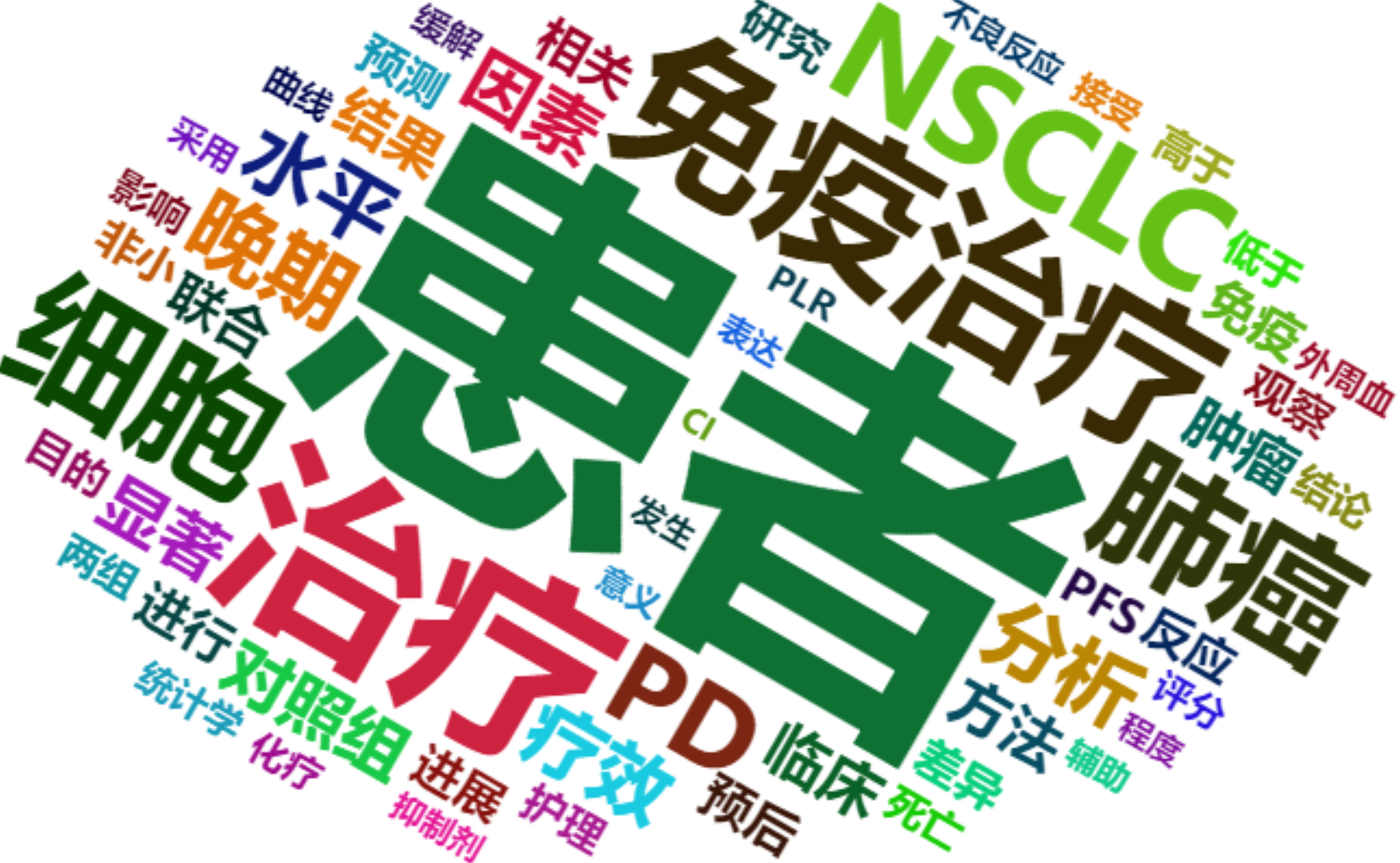

Figure 6: Fixed rotation

The direction of the words used in this figure is rotated 30 degrees clockwise. The maximum and minimum rotation angles need to be set to the same, and the rotation ratio is set to 1.

Tip

Key parameters: minRotation/maxRotation/rotateRatio

• minRotation: Minimum rotation angle.
• maxRotation: Maximum rotation angle.
• rotateRatio: The ratio of word rotation. rotateRatio = 1 will rotate all words.

Random rotation

# (2) Random rotation
RandomRotation <- wordcloud2(data = words_seg, size = 1, minRotation = -pi / 6,
                             maxRotation = pi / 6, rotateRatio = 0.8)
RandomRotation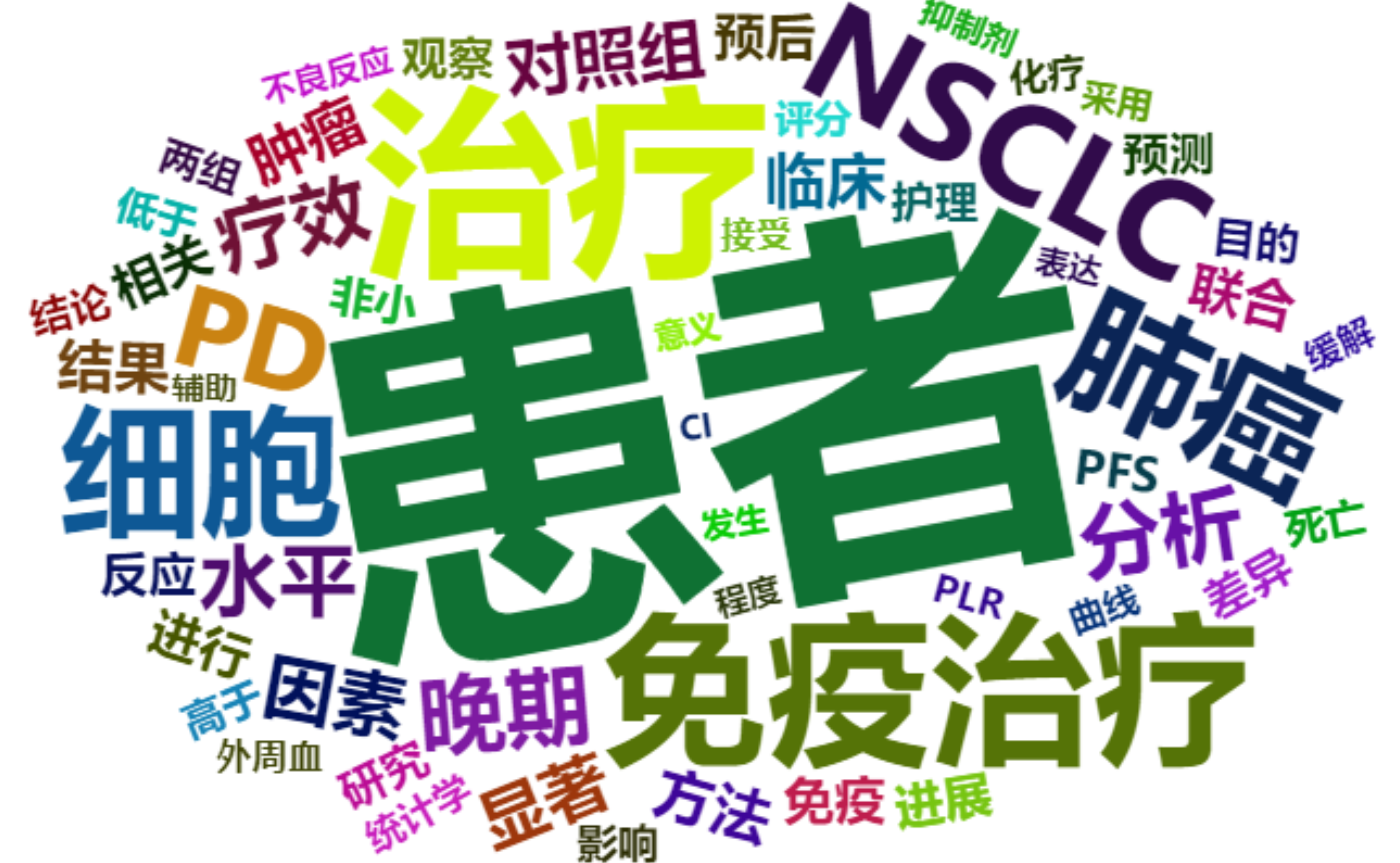

Figure 7: Random rotation

The rotation angle of this word cloud is between (-30°, 30°), the angle is selected randomly, and the rotation ratio is 0.8.

5. English word cloud

Using demoFreq data

# Using demoFreq data
EnglishWordcloud1 <- wordcloud2(data = demoFreq[1:75, ], size = 1)
EnglishWordcloud1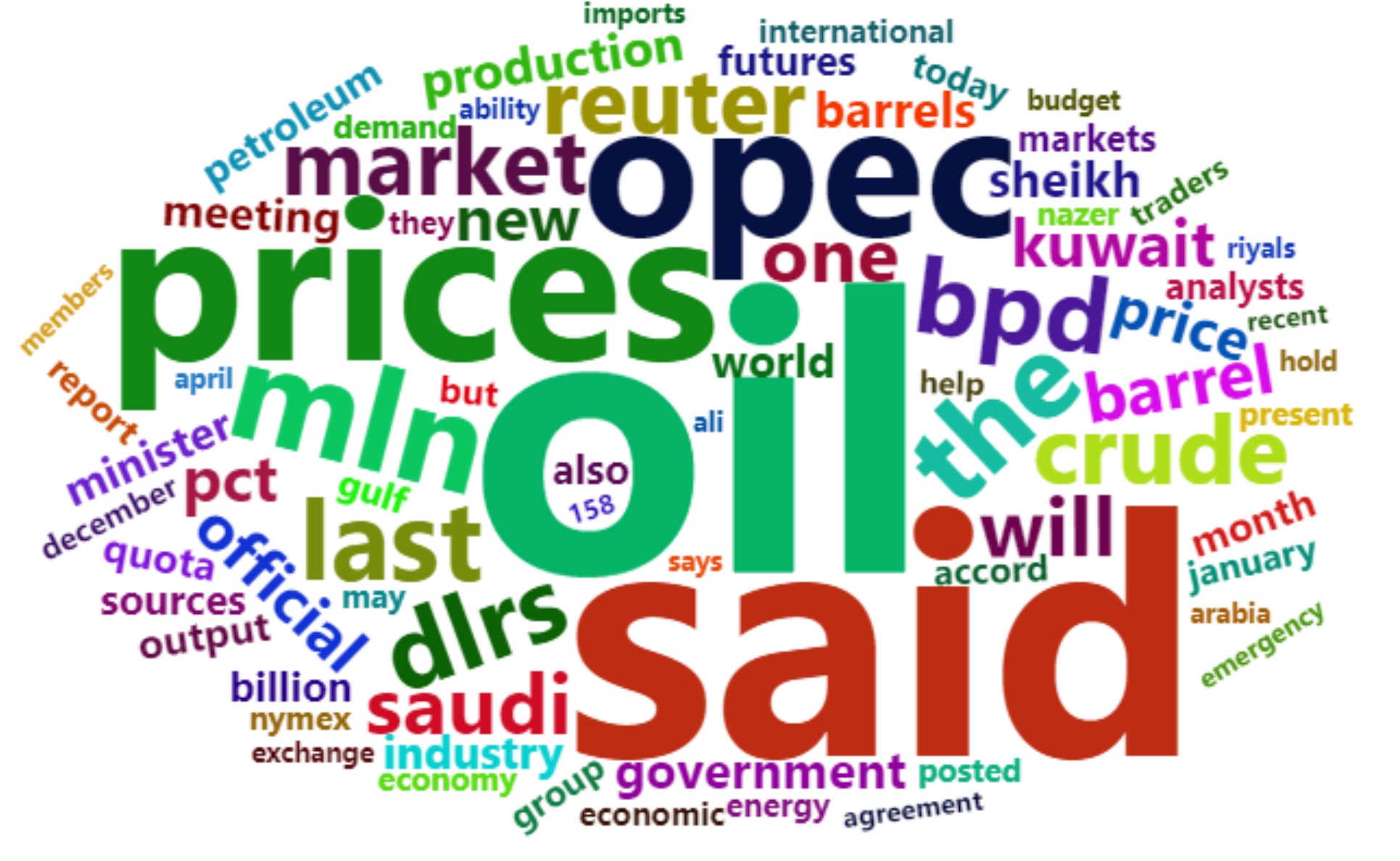

Figure 8: Using demoFreq data

The word cloud in this figure uses the first 75 items of the demoFreq dataset for plotting. The plotting code for the English word cloud and the Chinese word cloud is the same.

Use PubMed abstract text

# Use PubMed abstract text
EnglishWordcloud2 <- wordcloud2(data = words_english_sep1, size = 0.6)
EnglishWordcloud2

Figure 9: Use PubMed abstract text

The word cloud in the figure was drawn using PubMed abstract text and shows keywords for the topic of immunotherapy for lung cancer.

Applications

Figure 10: Applications of Wordcloud1

The visualization depicted in the figure shows that the bold, large font in the World Cloud visualization is intended to map the number of words that are the subject of each article abstract in maritime security research. The names of several countries, such as China, India, Indonesia, Australia, and the United States, are included in the World Cloud because most articles discuss certain countries or regions. [1]

Figure 11: Applications of Wordcloud2

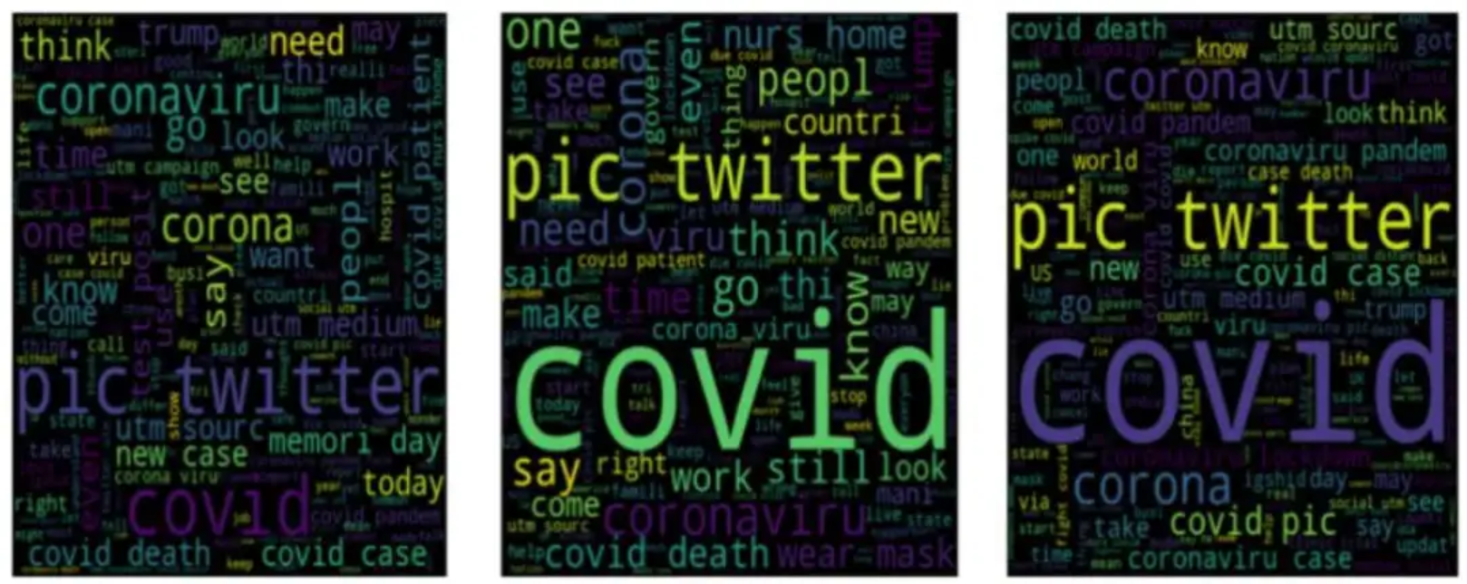
The three word clouds of DATA_SET 1 in the figure show the most frequently used words in positive, negative, and neutral emotions, respectively, verifying the author’s view that social media cannot provide netizens with appropriate courses for dealing with epidemics such as COVID-19. [2]

Figure 12: Applications of Wordcloud3

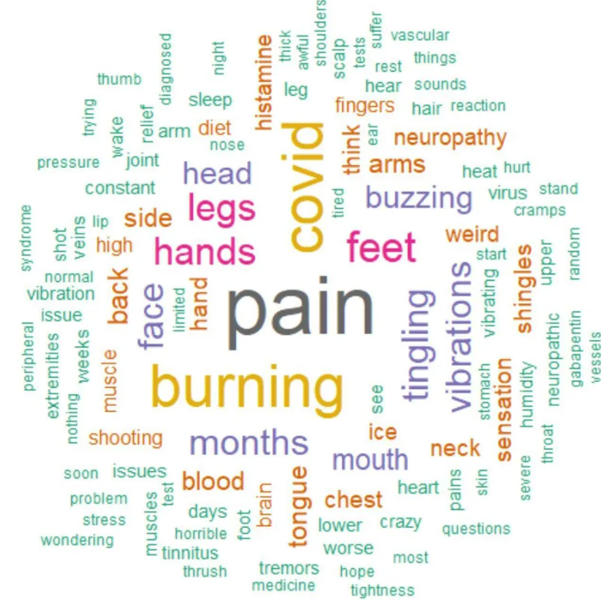
The word cloud shown here was created based on 162 comments from a Survivor Corps poll that asked respondents about vibrating or buzzing sensations and neuropathic pain. The word cloud shows that pain, burning, COVID-19, legs, hands, and feet were the most common terms mentioned in the comments. The word cloud includes terms related to sensations like burning and symptoms like shingles and thrush. [3]

Reference

[1] KISMARTINI K, YUSUF I M, SABILLA K R, et al. A bibliometric analysis of maritime security policy: Research trends and future agenda[J]. Heliyon, 2024,10(8): e28988.

[2] CHAKRABORTY K, BHATIA S, BHATTACHARYYA S, et al. Sentiment Analysis of COVID-19 tweets by Deep Learning Classifiers-A study to show how popularity is affecting accuracy in social media[J]. Appl Soft Comput, 2020,97: 106754.

[3] MASSEY D, SAWANO M, BAKER A D, et al. Characterisation of internal tremors and vibration symptoms[J]. BMJ Open, 2023,13(12): e77389.