# Install packages
if (!requireNamespace("data.table", quietly = TRUE)) {
  install.packages("data.table")
}
if (!requireNamespace("jsonlite", quietly = TRUE)) {
  install.packages("jsonlite")
}
if (!requireNamespace("circlize", quietly = TRUE)) {
  install.packages("circlize")
}
if (!requireNamespace("ComplexHeatmap", quietly = TRUE)) {
  BiocManager::install("ComplexHeatmap")
}
if (!requireNamespace("gtrellis", quietly = TRUE)) {
  remotes::install_github("jokergoo/gtrellis")
}
if (!requireNamespace("tidyverse", quietly = TRUE)) {
  install.packages("tidyverse")
}
if (!requireNamespace("ggplotify", quietly = TRUE)) {
  install.packages("ggplotify")
}
if (!requireNamespace("RColorBrewer", quietly = TRUE)) {
  install.packages("RColorBrewer")
}

# Load packages
library(data.table)
library(jsonlite)
library(circlize)
library(ComplexHeatmap)
library(gtrellis)
library(tidyverse)
library(ggplotify)
library(RColorBrewer)Gene Density
Note
Hiplot website
This page is the tutorial for source code version of the Hiplot Gene Density plugin. You can also use the Hiplot website to achieve no code ploting. For more information please see the following link:
Chrosome data visualization.
Setup
System Requirements: Cross-platform (Linux/MacOS/Windows)
Programming language: R
Dependent packages:
data.table;jsonlite;circlize;ComplexHeatmap;gtrellis;tidyverse;ggplotify;RColorBrewer
sessioninfo::session_info("attached")─ Session info ───────────────────────────────────────────────────────────────
setting value
version R version 4.6.0 (2026-04-24)
os Ubuntu 24.04.4 LTS
system x86_64, linux-gnu
ui X11
language (EN)
collate C.UTF-8
ctype C.UTF-8
tz UTC
date 2026-05-09
pandoc 3.1.3 @ /usr/bin/ (via rmarkdown)
quarto 1.9.37 @ /usr/local/bin/quarto
─ Packages ───────────────────────────────────────────────────────────────────
package * version date (UTC) lib source
BiocGenerics * 0.58.0 2026-04-28 [1] Bioconduc~
circlize * 0.4.18 2026-04-04 [1] RSPM
ComplexHeatmap * 2.28.0 2026-04-28 [1] Bioconduc~
data.table * 1.18.4 2026-05-06 [1] RSPM
dplyr * 1.2.1 2026-04-03 [1] RSPM
forcats * 1.0.1 2025-09-25 [1] RSPM
generics * 0.1.4 2025-05-09 [1] RSPM
GenomicRanges * 1.64.0 2026-04-28 [1] Bioconduc~
ggplot2 * 4.0.3.9000 2026-05-04 [1] Github (tidyverse/ggplot2@6870419)
ggplotify * 0.1.3 2025-09-20 [1] RSPM
gtrellis * 1.43.1 2026-05-04 [1] Github (jokergoo/gtrellis@d931194)
IRanges * 2.46.0 2026-04-28 [1] Bioconduc~
jsonlite * 2.0.0 2025-03-27 [1] RSPM
lubridate * 1.9.5 2026-02-04 [1] RSPM
purrr * 1.2.2 2026-04-10 [1] RSPM
RColorBrewer * 1.1-3 2022-04-03 [1] RSPM
readr * 2.2.0 2026-02-19 [1] RSPM
S4Vectors * 0.50.0 2026-04-28 [1] Bioconduc~
Seqinfo * 1.2.0 2026-04-28 [1] Bioconduc~
stringr * 1.6.0 2025-11-04 [1] RSPM
tibble * 3.3.1 2026-01-11 [1] RSPM
tidyr * 1.3.2 2025-12-19 [1] RSPM
tidyverse * 2.0.0 2023-02-22 [1] RSPM
[1] /home/runner/work/_temp/Library
[2] /opt/R/4.6.0/lib/R/site-library
[3] /opt/R/4.6.0/lib/R/library
* ── Packages attached to the search path.
──────────────────────────────────────────────────────────────────────────────Data Preparation
# Load data
data1 <- data.table::fread(jsonlite::read_json("https://hiplot.cn/ui/basic/gene-density/data.json")$exampleData$textarea[[1]])
data1 <- as.data.frame(data1)
data2 <- data.table::fread(jsonlite::read_json("https://hiplot.cn/ui/basic/gene-density/data.json")$exampleData$textarea[[2]])
data2 <- as.data.frame(data2)
# Convert data structure
chrNum <- str_replace(unique(data1$chr), "Chr|chr", "")
data1$chr <- factor(data1$chr, levels = paste0("Chr", chrNum))
data2$chr <- factor(data2$chr, levels = paste0("Chr", chrNum))
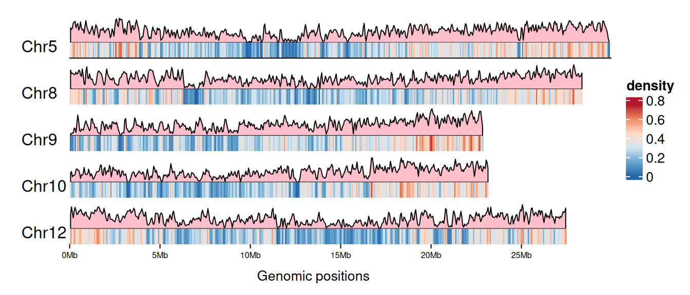
# Set window to calculate gene density
windows <- 100 * 1000 # default:100kb window size
gene_density <- genomicDensity(data2, window.size = windows)
gene_density$chr <- factor(gene_density$chr,
levels = paste0("Chr", chrNum)
)
# View data
head(data1) chr start end
1 Chr5 0 29958434
2 Chr8 0 28443022
3 Chr9 0 23012720
4 Chr10 0 23207287
5 Chr12 0 27531856head(data2) chr start end
1 Chr10 38648 40060
2 Chr10 45941 58338
3 Chr10 67119 72971
4 Chr10 75410 76305
5 Chr10 80964 82250
6 Chr10 94798 97746Visualization
# Set the palettes
palettes <- c("#B2182B","#EF8A62","#FDDBC7","#D1E5F0","#67A9CF","#2166AC")
col_fun <- colorRamp2(
  seq(0, max(gene_density[[4]]), length = 6), rev(palettes)
  )
cm <- ColorMapping(col_fun = col_fun)
# Set the Legend
lgd <- color_mapping_legend(
  cm, plot = F, title = "density", color_bar = "continuous"
  )
# Plot
p <- as.ggplot(function() {
  gtrellis_layout(
    data1, n_track = 2, ncol = 1, byrow = FALSE,
    track_axis = FALSE, add_name_track = FALSE,
    xpadding = c(0.1, 0), gap = unit(1, "mm"),
    track_height = unit.c(unit(1, "null"), unit(4, "mm")),
    track_ylim = c(0, max(gene_density[[4]]), 0, 1),
    border = FALSE, asist_ticks = FALSE,
    legend = lgd
    )
  # Add gene area map track
  add_lines_track(gene_density, gene_density[[4]],
                  area = TRUE, gp = gpar(fill = "pink"))
  # Add gene density heatmap track
  add_heatmap_track(gene_density, gene_density[[4]], fill = col_fun)
  add_track(track = 2, clip = FALSE, panel_fun = function(gr) {
    chr <- get_cell_meta_data("name")
    if (chr == paste("Chr", length(chrNum), sep = "")) {
      grid.lines(get_cell_meta_data("xlim"), unit(c(0, 0), "npc"),
                 default.units = "native")
      }
    grid.text(chr, x = 0.01, y = 0.38, just = c("left", "bottom"))
    })
  circos.clear()
  })

p