Faceted Plots (Julia)

🤖 AI Skill — Download the Bizard unified skill for your AI assistant ⬇️ Download Skill ZIP

🔌 MCP Server — Let AI agents (Claude Code, Cursor, …) query Bizard live: claude mcp add bizard -- npx @openbiox/bizard-mcp — or the free hosted instance (no install, faster from mainland China): claude mcp add --transport http bizard http://biotree.top:38123/bizard-mcp/mcp 📖 MCP Docs

📖 Cite Bizard — if Bizard helps your research, please cite: Li, K., Zheng, H., Huang, K., et al. (2026). Bizard: A Community-Driven Platform for Accelerating and Enhancing Biomedical Data Visualization. iMetaMed, e70038. 🔗 DOI / BibTeX

Faceting splits one dataset into a grid of panels by categorical variables, holding every panel on identical axes so group differences read as shape differences. In Julia the grammar-of-graphics layer AlgebraOfGraphics composes faceted specifications from a mapping — the closest Julia equivalent to ggplot faceting or seaborn’s relplot.

Example

Setup

• System Requirements: Cross-platform (Linux/MacOS/Windows)
• Programming Language: Julia
• Dependencies: CairoMakie, AlgebraOfGraphics, DataFrames, Statistics

using CairoMakie
using AlgebraOfGraphics
using DataFrames
using Statistics
using Random

Data Preparation

We simulate a longitudinal treatment study in long format — 4 genotypes × 2 arms × 6 weekly measurements — one row per observation, the shape AlgebraOfGraphics expects.

Random.seed!(201)

genotypes = ["WT", "HET", "KO", "RES"]
rates = Dict(g => 0.10 + 0.08 * (3 - i) for (i, g) in enumerate(genotypes))
rows = []
for geno in genotypes
    for arm in ["Vehicle", "Treatment"]
        rate = rates[geno] + (arm == "Treatment" ? 0.0 : -0.05)
        for mouse in 1:8, week in 0:5
            push!(rows, (Genotype = geno, Arm = arm, Week = week,
                         Score = 1 + 2.4 * rate * week / 5 + 0.12 * randn()))
        end
    end
end
long = DataFrame(rows)

384×4 DataFrame

359 rows omitted

Row	Genotype	Arm	Week	Score
	String	String	Int64	Float64
1	WT	Vehicle	0	0.996337
2	WT	Vehicle	1	1.09882
3	WT	Vehicle	2	1.30855
4	WT	Vehicle	3	1.17022
5	WT	Vehicle	4	1.34779
6	WT	Vehicle	5	1.55968
7	WT	Vehicle	0	1.15025
8	WT	Vehicle	1	1.13707
9	WT	Vehicle	2	1.11064
10	WT	Vehicle	3	1.38315
11	WT	Vehicle	4	1.42207
12	WT	Vehicle	5	1.76371
13	WT	Vehicle	0	1.11001
⋮	⋮	⋮	⋮	⋮
373	RES	Treatment	0	1.18669
374	RES	Treatment	1	0.97793
375	RES	Treatment	2	1.11329
376	RES	Treatment	3	0.927396
377	RES	Treatment	4	0.995892
378	RES	Treatment	5	0.856548
379	RES	Treatment	0	1.15491
380	RES	Treatment	1	0.97661
381	RES	Treatment	2	1.25163
382	RES	Treatment	3	1.17638
383	RES	Treatment	4	1.04982
384	RES	Treatment	5	0.966681

Visualization

Faceted Trajectories

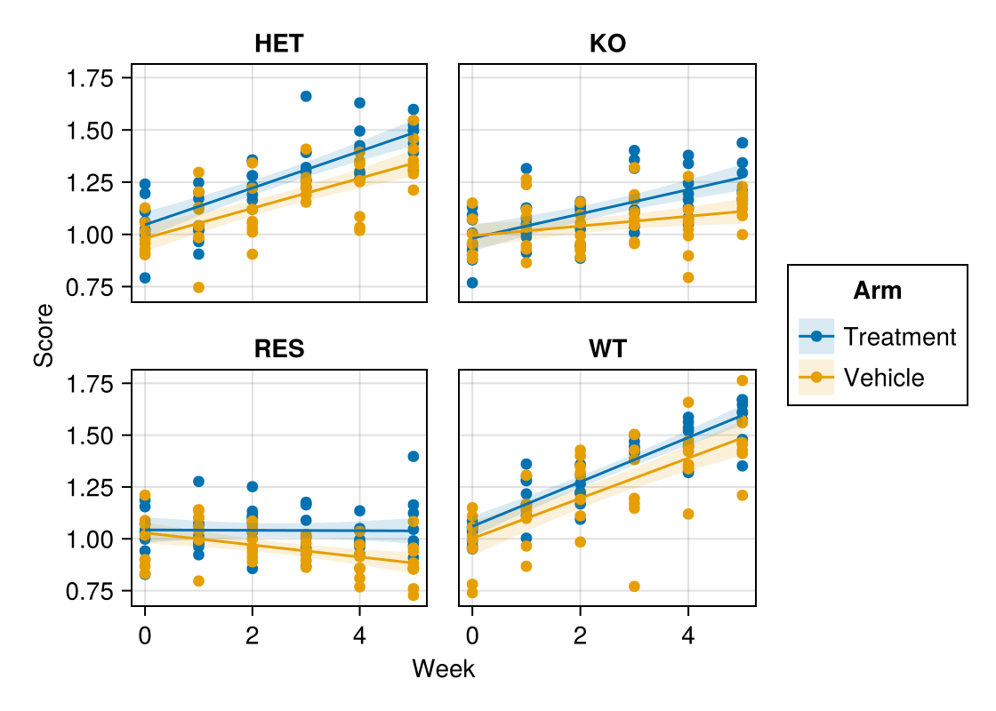
mapping carries the aesthetic assignment (layout facets the grid); combining with a smoothed visual line layer builds the panel in one pipeline.

spec = data(long) * mapping(:Week, :Score, color = :Arm,
                            layout = :Genotype) *
       visual(Scatter) +
       data(long) * mapping(:Week, :Score, color = :Arm,
                            layout = :Genotype) * linear()

fg = draw(spec; figure = (size = (560, 400),))
fg

Figure 1: Response trajectories faceted by genotype, coloured by arm

Distribution Facets

The same grammar swaps layers for a histogram + density analysis; mapping decides what, the analysis decides how.

final = long[long.Week .== 5, :]

hist_spec = data(final) * mapping(:Score, layout = :Genotype, color = :Genotype) *
            histogram(bins = 14) +
            data(final) * mapping(:Score, layout = :Genotype, color = :Genotype) *
            AlgebraOfGraphics.density()

fg = draw(hist_spec; figure = (size = (560, 380),))
fg

Figure 2: Final-week score distributions faceted by genotype

References

1. AlgebraOfGraphics development team. AlgebraOfGraphics.jl documentation. https://aog.makie.org/
2. Danisch, S., & Krumbiegel, J. (2021). Makie.jl: Flexible high-performance data visualization for Julia. Journal of Open Source Software, 6(65), 3349.