# Install packages
if (!requireNamespace("data.table", quietly = TRUE)) {
  install.packages("data.table")
}
if (!requireNamespace("jsonlite", quietly = TRUE)) {
  install.packages("jsonlite")
}
if (!requireNamespace("ggstatsplot", quietly = TRUE)) {
  install.packages("ggstatsplot")
}
if (!requireNamespace("ggplot2", quietly = TRUE)) {
  install.packages("ggplot2")
}
if (!requireNamespace("cowplot", quietly = TRUE)) {
  install.packages("cowplot")
}

# Load packages
library(data.table)
library(jsonlite)
library(ggstatsplot)
library(ggplot2)
library(cowplot)Betweenstats
Note
Hiplot website
This page is the tutorial for source code version of the Hiplot Betweenstats plugin. You can also use the Hiplot website to achieve no code ploting. For more information please see the following link:
Setup
System Requirements: Cross-platform (Linux/MacOS/Windows)
Programming language: R
Dependent packages:
data.table;jsonlite;ggstatsplot;ggplot2;cowplot
sessioninfo::session_info("attached")─ Session info ───────────────────────────────────────────────────────────────
setting value
version R version 4.6.0 (2026-04-24)
os Ubuntu 24.04.4 LTS
system x86_64, linux-gnu
ui X11
language (EN)
collate C.UTF-8
ctype C.UTF-8
tz UTC
date 2026-05-09
pandoc 3.1.3 @ /usr/bin/ (via rmarkdown)
quarto 1.9.37 @ /usr/local/bin/quarto
─ Packages ───────────────────────────────────────────────────────────────────
package * version date (UTC) lib source
cowplot * 1.2.0 2025-07-07 [1] RSPM
data.table * 1.18.4 2026-05-06 [1] RSPM
ggplot2 * 4.0.3.9000 2026-05-04 [1] Github (tidyverse/ggplot2@6870419)
ggstatsplot * 1.0.0 2026-04-23 [1] RSPM
jsonlite * 2.0.0 2025-03-27 [1] RSPM
[1] /home/runner/work/_temp/Library
[2] /opt/R/4.6.0/lib/R/site-library
[3] /opt/R/4.6.0/lib/R/library
* ── Packages attached to the search path.
──────────────────────────────────────────────────────────────────────────────Data Preparation
# Load data
data <- data.table::fread(jsonlite::read_json("https://hiplot.cn/ui/basic/ggbetweenstats/data.json")$exampleData$textarea[[1]])
data <- as.data.frame(data)

# Convert data structure
axis <- c("mpaa", "length", "genre")
data[, axis[1]] <- factor(data[, axis[1]], levels = unique(data[, axis[1]]))
data[, axis[3]] <- factor(data[, axis[3]], levels = unique(data[, axis[3]]))

# View data
head(data)
title year
1 Lord of the Rings: The Return of the King, The 2003
2 Lord of the Rings: The Fellowship of the Ring, The 2001
3 Lord of the Rings: The Two Towers, The 2002
4 Star Wars 1977
5 Star Wars: Episode V - The Empire Strikes Back 1980
6 Dr. Strangelove or: How I Learned to Stop Worrying and Love the Bomb 1964
length budget rating votes mpaa genre
1 251 94.0 9.0 103631 PG-13 Action
2 208 93.0 8.8 157608 PG-13 Action
3 223 94.0 8.8 114797 PG-13 Action
4 125 11.0 8.8 134640 PG Action
5 129 18.0 8.8 103706 PG Action
6 93 1.8 8.7 63471 PG ComedyVisualization
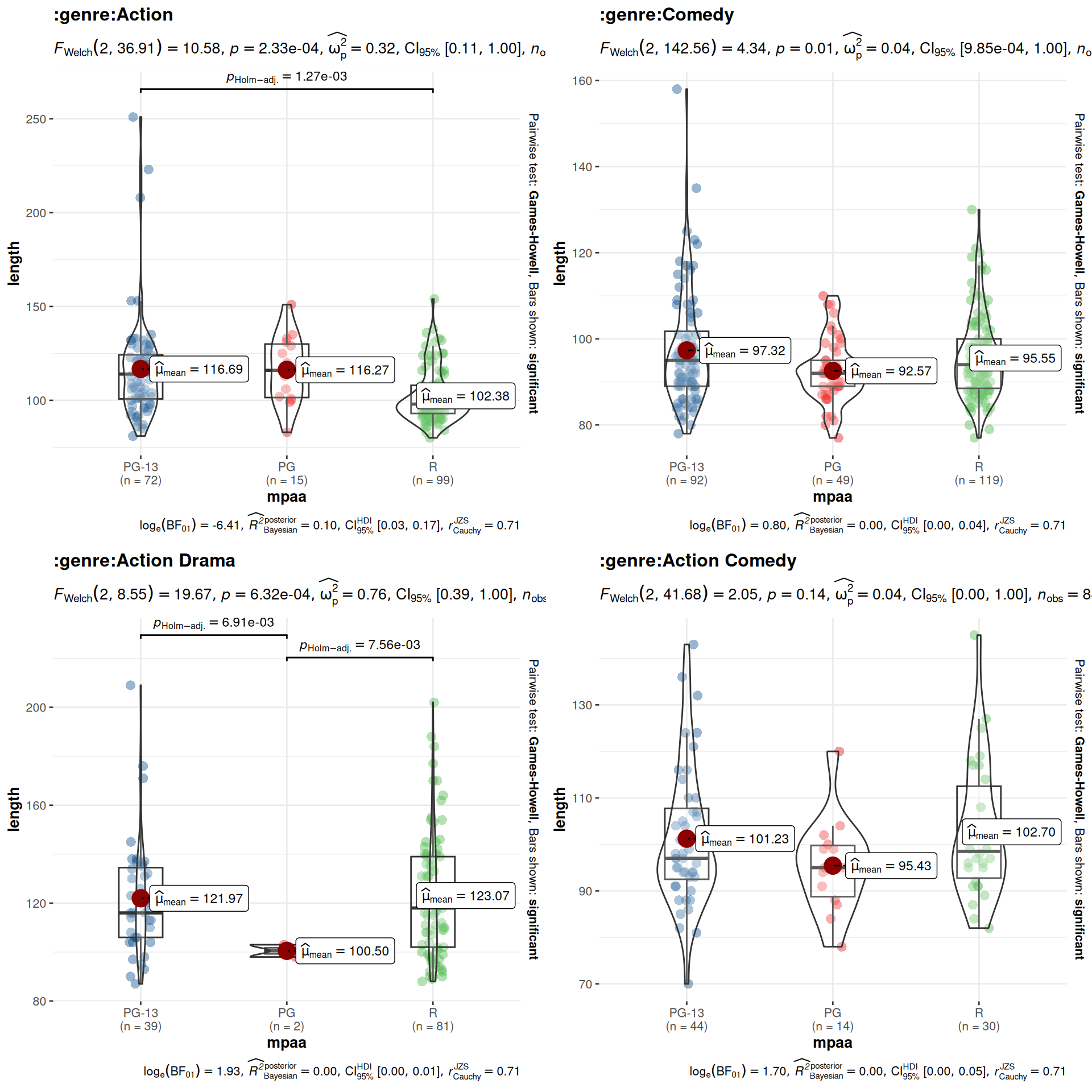
# Betweenstats
g <- unique(data[,axis[3]])
plist <- list()
for (i in 1:length(g)) {
  fil <- data[,axis[3]] == g[i]
  plist[[i]] <- ggbetweenstats(
    data = data[fil,], x = mpaa, y = length,
    title= paste('', axis[3], g[i], sep = ':'),
    p.adjust.method = "holm",
    plot.type = "boxviolin",
    pairwise.comparisons = T,
    pairwise.display = "significant",
    effsize.type = "unbiased",
    notch = T,
    type = "parametric",
    plotgrid.args = list(ncol = 2)) +
    scale_color_manual(values = c("#00468BFF","#ED0000FF","#42B540FF"))
}
p <- plot_grid(plotlist = plist, ncol = 2)

p