# Installing necessary packages
if (!requireNamespace("Rtsne", quietly = TRUE)) {
  install.packages("Rtsne")
}
if (!requireNamespace("patchwork", quietly = TRUE)) {
  install.packages("patchwork")
}

# Load packages
library(Rtsne)
library(ggplot2)
library(dplyr)
library(patchwork)t-SNE Plot
t-distributed stochastic neighbor embedding (t-SNE) projects high-dimensional data — thousands of genes per cell, hundreds of features per sample — onto a 2-D map that keeps neighboring observations close [1]. It is the workhorse embedding of single-cell genomics: cell types that separate in 20,000-dimensional expression space separate into visual islands in t-SNE space, making population structure visible at a glance.
t-SNE answers a structure question (“how many populations are there, and who is next to whom”), not a distance question: inter-cluster distances and cluster sizes on the map carry no global meaning, and the map changes with the perplexity hyperparameter and the random seed. PCA, by contrast, keeps global geometry but only linear structure — the two are complementary, and the standard practice is to run t-SNE on the top principal components rather than on raw features [2].
This tutorial covers four practical workflows with Rtsne [3]:
- A basic t-SNE map of a simulated single-cell expression matrix;
- How
perplexityreshapes the map (the one parameter to always check); - t-SNE versus PCA on the same data;
- Overlaying a marker gene’s expression onto the map.
Example
Setup
System Requirements: Cross-platform (Linux/MacOS/Windows)
Programming language: R
Dependent packages:
Rtsne;ggplot2;dplyr;patchwork
sessioninfo::session_info("attached")─ Session info ───────────────────────────────────────────────────────────────
setting value
version R version 4.6.2 (2026-10-29)
os Ubuntu 24.04.5 LTS
system x86_64, linux-gnu
ui X11
language (EN)
collate C.UTF-8
ctype C.UTF-8
tz UTC
date 2026-10-31
pandoc 3.1.3 @ /usr/bin/ (via rmarkdown)
quarto 1.10.20 @ /usr/local/bin/quarto
─ Packages ───────────────────────────────────────────────────────────────────
! package * version date (UTC) lib source
P dplyr * 1.2.1 2026-04-03 [?] RSPM
P ggplot2 * 4.0.3.9000 2026-10-30 [?] Github (tidyverse/ggplot2@b638d65)
P patchwork * 1.3.2 2025-08-25 [?] RSPM
P Rtsne * 0.17 2023-12-07 [?] RSPM
[1] /home/runner/.cache/R/renv/library/Bizard-5140bdc6/linux-ubuntu-noble/R-4.6/x86_64-pc-linux-gnu
[2] /home/runner/work/_temp/Library
[3] /opt/R/4.6.2/lib/R/library
* ── Packages attached to the search path.
P ── Loaded and on-disk path mismatch.
──────────────────────────────────────────────────────────────────────────────Data Preparation
We simulate a scRNA-seq-like log-expression matrix: 1,200 cells from four populations (CD4 T cells, B cells, NK cells, monocytes) × 200 genes, where each population expresses a private block of 20 marker genes. The four populations differ in marker blocks only — a structure t-SNE should recover as four islands.
set.seed(251)

n_per   <- 300
types   <- c("CD4 T cells", "B cells", "NK cells", "Monocytes")
n_genes <- 200

base <- matrix(rnorm(n_per * length(types) * n_genes, 0, 0.6),
               nrow = n_per * length(types), ncol = n_genes,
               dimnames = list(NULL, paste0("Gene", 1:n_genes)))
ct <- rep(types, each = n_per)
markers <- list("CD4 T cells" = 1:20, "B cells" = 21:40,
                "NK cells" = 41:60, "Monocytes" = 61:80)
for (t in types) {
  idx <- which(ct == t)
  base[idx, markers[[t]]] <- base[idx, markers[[t]]] + 2.5
}
expr <- pmax(base + rnorm(length(base), 0, 0.3), 0)

# Standard practice: run t-SNE on the top principal components, not raw genes
pcs <- prcomp(expr, rank. = 30)$x[, 1:30]
Visualization
1. Basic t-SNE Map
set.seed(251)                       # t-SNE is stochastic: fix the seed
tsne30 <- Rtsne(pcs, dims = 2, perplexity = 30, pca = FALSE, verbose = FALSE)

d30 <- data.frame(tSNE1 = tsne30$Y[, 1], tSNE2 = tsne30$Y[, 2], celltype = ct)
cent <- d30 |>
  group_by(celltype) |>
  summarise(tSNE1 = mean(tSNE1), tSNE2 = mean(tSNE2))

pal <- c("#4E79A7", "#F28E2B", "#E15759", "#76B7B2")
p1 <- ggplot(d30, aes(tSNE1, tSNE2, color = celltype)) +
  geom_point(size = 0.7, alpha = 0.8) +
  geom_text(data = cent, aes(tSNE1, tSNE2, label = celltype),
            inherit.aes = FALSE, color = "black",
            fontface = "bold", size = 3.5, vjust = -1.2) +
  scale_color_manual(values = pal) +
  labs(x = "t-SNE 1", y = "t-SNE 2") +
  theme_bw(base_size = 11) +
  theme(legend.position = "none")
p1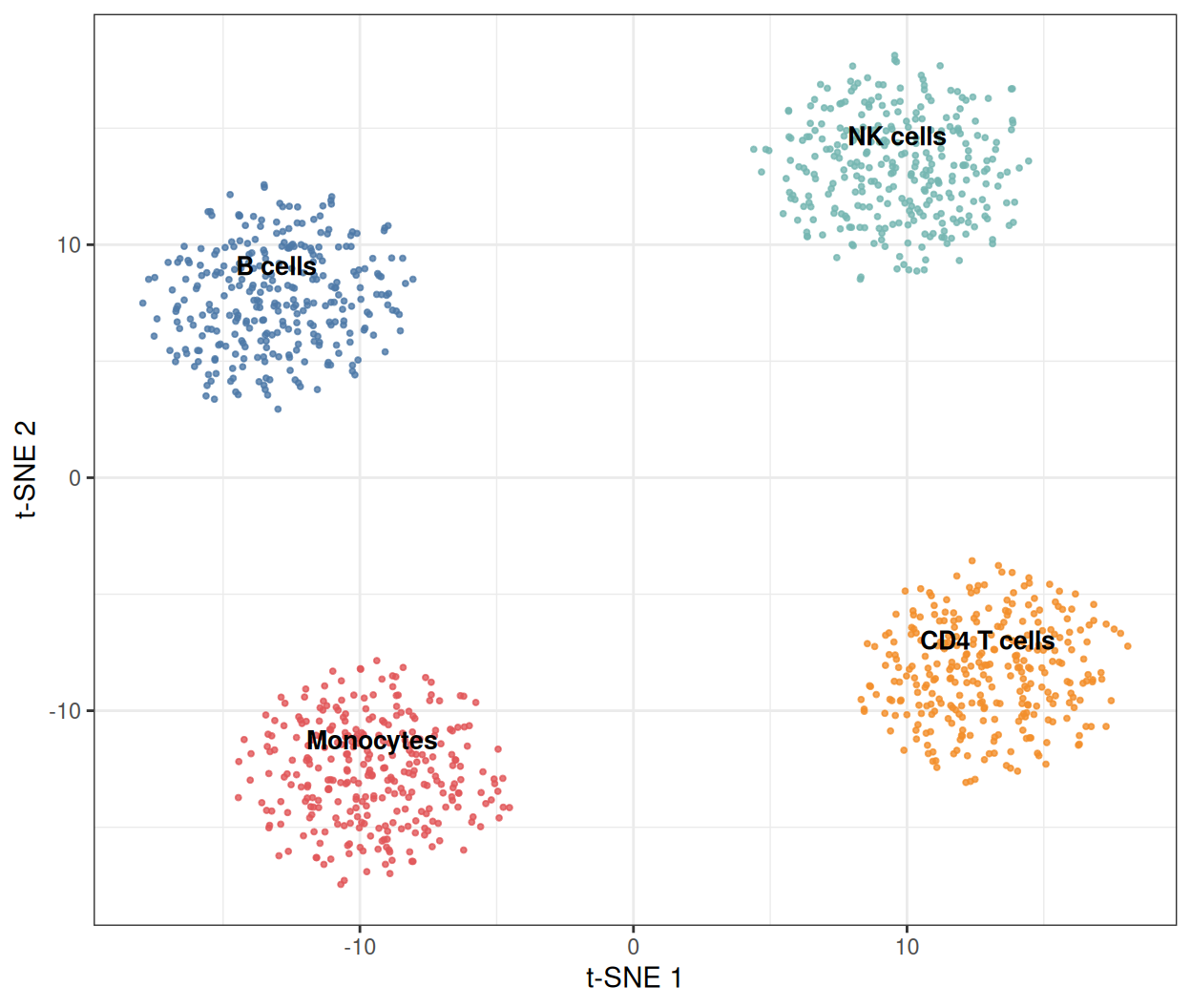
Four islands, one per population. Note the axes: t-SNE dimensions have no units and no fixed orientation — rerunning with a different seed rotates and mirrors the map while preserving the neighborhood structure.
2. The Perplexity Trade-off
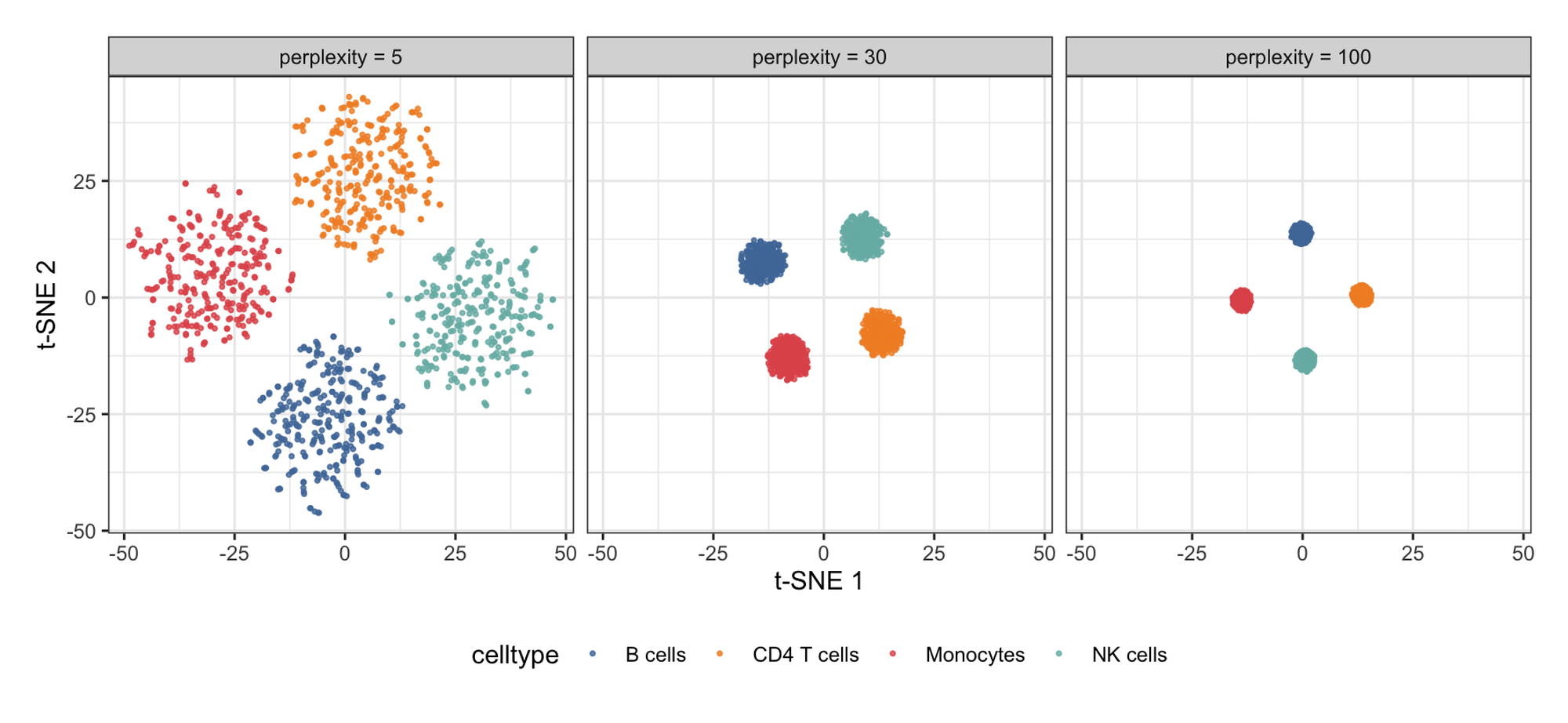
perplexity (roughly, the effective number of neighbors each point considers) is the single most consequential parameter. Low values resolve local detail; high values merge populations; typical choices are 5–50 for thousands of cells, and the honest report shows the map is stable across a range.
mk <- function(ppl) {
  set.seed(251)
  ts <- Rtsne(pcs, dims = 2, perplexity = ppl, pca = FALSE, verbose = FALSE)
  data.frame(tSNE1 = ts$Y[, 1], tSNE2 = ts$Y[, 2], celltype = ct, perplexity = ppl)
}
dfp <- bind_rows(mk(5), mk(30), mk(100))

ggplot(dfp, aes(tSNE1, tSNE2, color = celltype)) +
  geom_point(size = 0.6, alpha = 0.8) +
  facet_wrap(~perplexity, labeller = labeller(
    perplexity = function(x) paste0("perplexity = ", x))) +
  scale_color_manual(values = pal) +
  labs(x = "t-SNE 1", y = "t-SNE 2") +
  theme_bw(base_size = 11) +
  theme(legend.position = "bottom")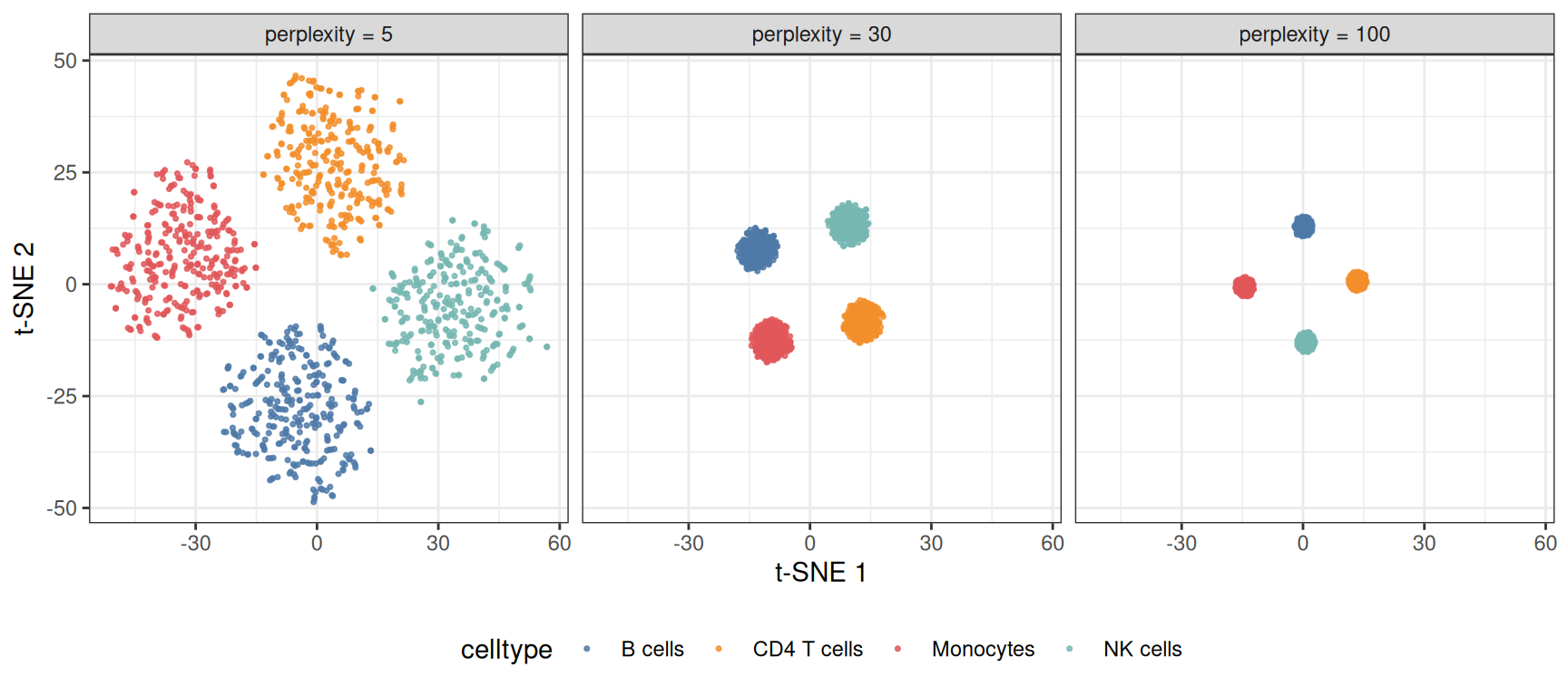
At perplexity 5 the marker-block noise fragments each population into sub-clusters; at 100 the four populations compress into featureless blobs. Interpret every t-SNE figure with its perplexity in the caption.
3. t-SNE versus PCA
pdf <- data.frame(PC1 = pcs[, 1], PC2 = pcs[, 2], celltype = ct)
p3a <- ggplot(pdf, aes(PC1, PC2, color = celltype)) +
  geom_point(size = 0.6, alpha = 0.8) +
  scale_color_manual(values = pal) +
  labs(x = "PC 1", y = "PC 2", title = "PCA (linear)") +
  theme_bw(base_size = 11) + theme(legend.position = "none")
p3b <- p1 + labs(title = "t-SNE (nonlinear)")

p3a / p3b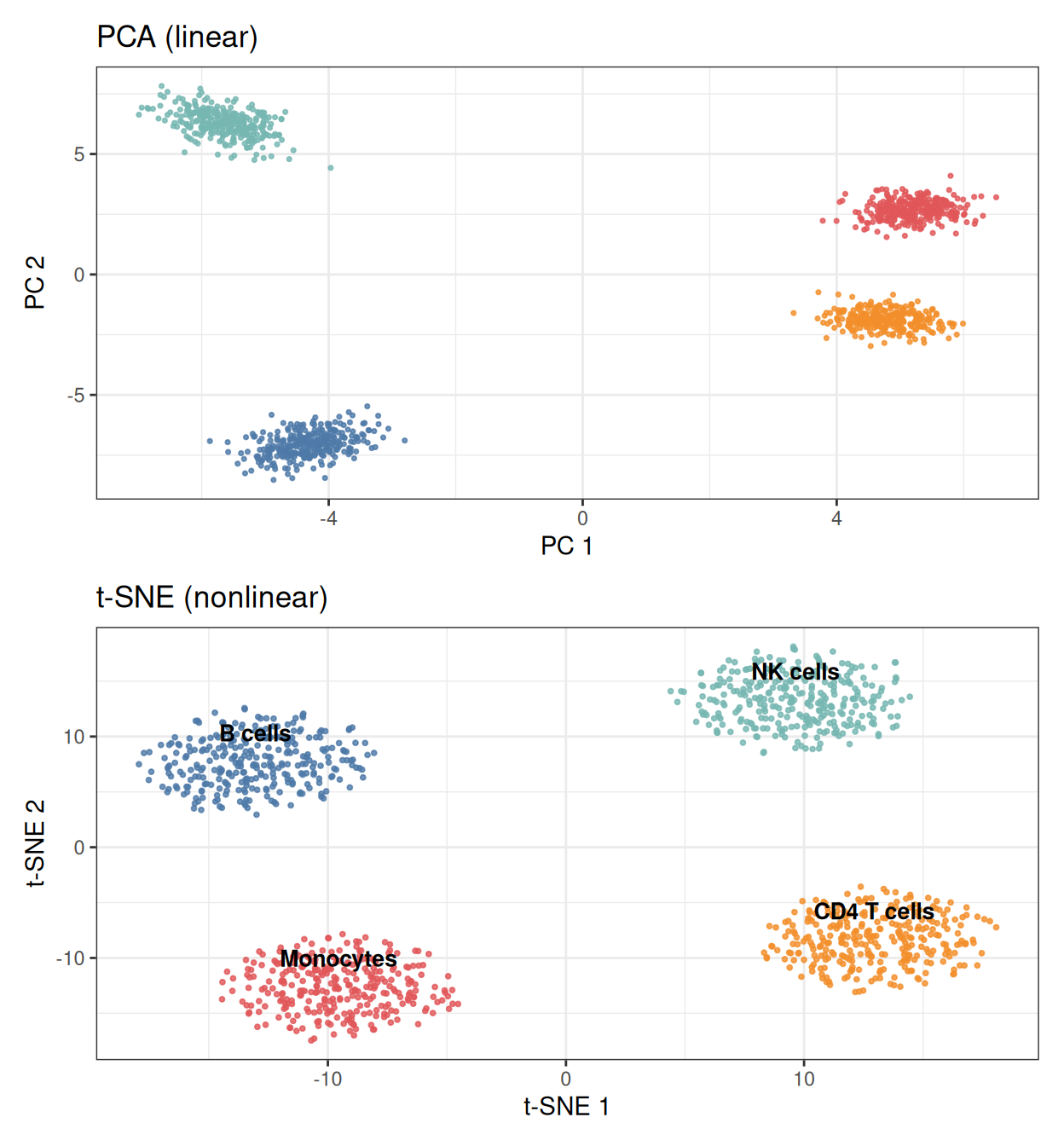
PCA keeps the populations at their true relative sizes and positions; t-SNE equalizes cluster areas and stretches the space so neighbors touch. Use PCA when magnitudes and gradients matter (trajectory endpoints, batch shifts), t-SNE when population discovery matters.
4. Overlaying Marker Expression
dfm <- d30
dfm$marker <- expr[, "Gene1"]          # CD4 T cell marker block member

ggplot(dfm, aes(tSNE1, tSNE2, color = marker)) +
  geom_point(size = 0.7, alpha = 0.9) +
  scale_color_gradient(low = "#EEEEEE", high = "#B2182B", name = "Gene1") +
  labs(x = "t-SNE 1", y = "t-SNE 2") +
  theme_bw(base_size = 11)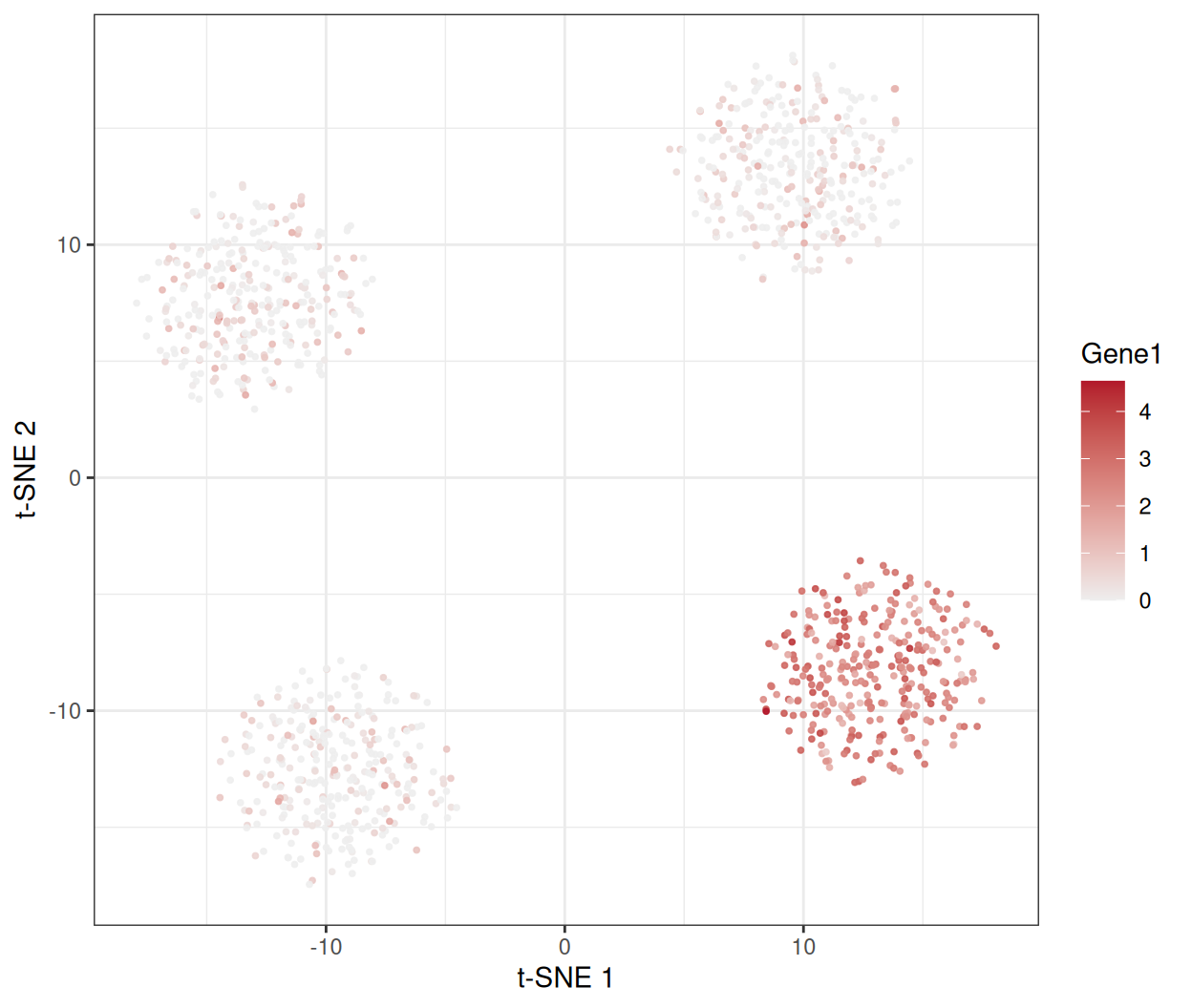
Painting per-cell values (gene expression, cluster score, QC metrics) onto the map is how t-SNE figures earn their interpretation.
TipPractice tips
- Always
set.seed()beforeRtsne()— the optimization is stochastic, and unseeded maps are unreproducible. - Feed the top 20–50 PCs, not raw features: denoising first is the difference between structure and noise (and it is much faster).
- Report the perplexity; check at least two values before trusting a cluster boundary.
- Never read global distances: two islands far apart on the map are not necessarily “more different” than two nearby islands.
- t-SNE cannot embed new samples into an existing map — use UMAP for that, or refit.
Application
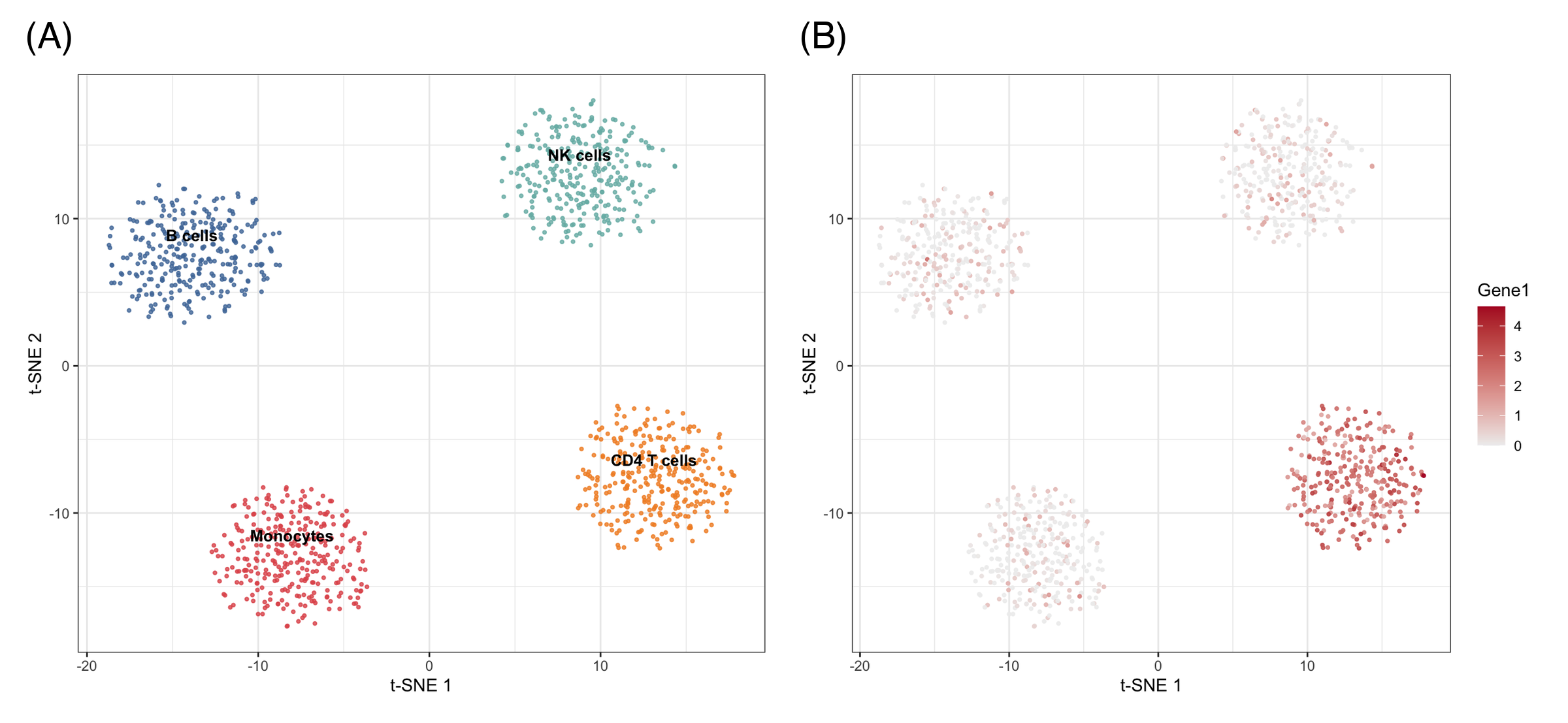
t-SNE maps are the front-page figure of single-cell papers (cell-type atlases, tumor immune infiltrates) and appear whenever many features must be reduced to a population map: cytometry panels, methylation profiles, and drug-screen morphology. The panel below mirrors a typical publication layout: (A) the perplexity check and (B) the population map with marker overlay.
Reference
[1] van der Maaten L, Hinton G. Visualizing data using t-SNE. J Mach Learn Res. 2008;9:2579-2605.
[2] Kobak D, Berens P. The art of using t-SNE for single-cell transcriptomics. Nat Commun. 2019;10:5416. doi:10.1038/s41467-019-13056-x
[3] Krijthe JH. Rtsne: t-Distributed Stochastic Neighbor Embedding using Barnes-Hut implementation. R package version 0.17. 2015. https://github.com/jkrijthe/Rtsne