# Installing necessary packages
if (!requireNamespace("pROC", quietly = TRUE)) {
  install.packages("pROC")
}
if (!requireNamespace("plotROC", quietly = TRUE)) {
  install.packages("plotROC")
}
if (!requireNamespace("timeROC", quietly = TRUE)) {
  install.packages("timeROC")
}

# Load packages
library(survival)
library(dplyr)
library(ggplot2)
library(pROC)
library(plotROC)
library(timeROC)ROC Curve
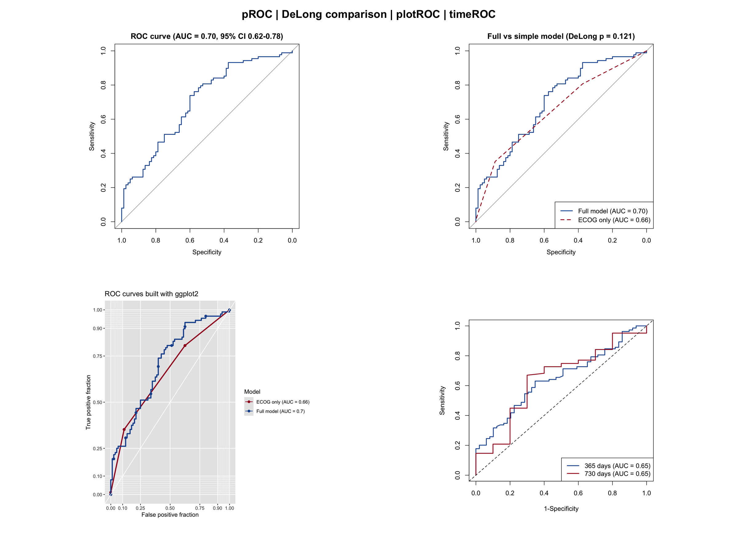
The receiver operating characteristic (ROC) curve evaluates the discrimination of a binary classifier — most commonly a clinical prediction model — across all possible decision thresholds. It plots sensitivity (true-positive rate) against 1 − specificity (false-positive rate), and is summarized by the area under the curve (AUC): 0.5 indicates discrimination no better than chance and 1.0 indicates perfect discrimination. In clinical research, ROC analysis is one of the standard tools for reporting the performance of diagnostic and prognostic models, together with calibration curves and decision curve analysis (see the companion tutorials).
This tutorial covers four practical ROC workflows in R:
- Basic ROC with AUC and bootstrap confidence interval (
pROC); - Comparing the discrimination of two models with the DeLong test (
pROC); - Publication-style ROC curves with automatically reported AUCs (
plotROC); - Time-dependent ROC for survival outcomes at fixed horizons (
timeROC).
Example
Setup
System Requirements: Cross-platform (Linux/MacOS/Windows)
Programming language: R
Dependent packages:
survival;dplyr;pROC;plotROC;timeROC;ggplot2
sessioninfo::session_info("attached")─ Session info ───────────────────────────────────────────────────────────────
setting value
version R version 4.6.1 (2026-06-24)
os Ubuntu 24.04.5 LTS
system x86_64, linux-gnu
ui X11
language (EN)
collate C.UTF-8
ctype C.UTF-8
tz UTC
date 2026-10-29
pandoc 3.1.3 @ /usr/bin/ (via rmarkdown)
quarto 1.10.19 @ /usr/local/bin/quarto
─ Packages ───────────────────────────────────────────────────────────────────
! package * version date (UTC) lib source
P dplyr * 1.2.1 2026-04-03 [?] RSPM
P ggplot2 * 4.0.3.9000 2026-10-26 [?] Github (tidyverse/ggplot2@b638d65)
P plotROC * 2.3.3 2025-08-25 [?] RSPM
P pROC * 1.19.1 2026-08-27 [?] RSPM
survival * 3.8-6 2026-01-16 [3] CRAN (R 4.6.1)
timeROC * 0.4.1 2026-04-10 [1] RSPM
[1] /home/runner/.cache/R/renv/library/Bizard-5140bdc6/linux-ubuntu-noble/R-4.6/x86_64-pc-linux-gnu
[2] /home/runner/work/_temp/Library
[3] /opt/R/4.6.1/lib/R/library
* ── Packages attached to the search path.
P ── Loaded and on-disk path mismatch.
──────────────────────────────────────────────────────────────────────────────Data Preparation
We use the built-in lung data set from the survival package (North Central Cancer Treatment Group lung cancer trial) [1]. We define a binary endpoint — death within the first year of follow-up — and fit two logistic models: a full model using five covariates and a simple model using only the ECOG performance score. We also build a Cox model to derive a continuous risk score for the time-dependent ROC analysis.
# The lung data set ships with the survival package
data(lung, package = "survival")

lung2 <- lung %>%
  filter(complete.cases(age, sex, ph.ecog, ph.karno, pat.karno, meal.cal, wt.loss)) %>%
  mutate(y1y = as.integer(time < 365 & status == 2))  # death within 365 days
  # Caveat: patients censored before day 365 are counted as non-events; for
  # real analyses prefer restricting to >=365 days of follow-up or using
  # censoring-aware methods (cf. the time-dependent ROC below).

cat("Patients:", nrow(lung2), " 1-year deaths:", sum(lung2$y1y), "\n")
Patients: 168 1-year deaths: 88 # Two logistic models for 1-year mortality
m_full <- glm(y1y ~ age + sex + ph.ecog + meal.cal + wt.loss,
data = lung2, family = binomial)
m_simple <- glm(y1y ~ ph.ecog, data = lung2, family = binomial)
# A continuous risk score from a Cox model (used for time-dependent ROC)
cph0 <- coxph(Surv(time, status) ~ age + sex + ph.ecog + wt.loss, data = lung2)
lung2$risk_score <- as.numeric(predict(cph0, type = "risk"))
# Store each model's predicted probability as a column (required by melt_roc)
lung2$risk_full <- fitted(m_full)
lung2$risk_ecog <- fitted(m_simple)Visualization
1. Basic ROC Curve with AUC and Confidence Interval
roc_full <- roc(lung2$y1y, fitted(m_full), quiet = TRUE)
set.seed(2026)  # keep the bootstrap CI reproducible across renders
ci_full  <- ci.auc(roc_full, method = "bootstrap", boot.n = 1000)

plot(roc_full, col = "#2166AC", lwd = 2,
     main = sprintf("ROC curve (AUC = %.2f, 95%% CI %.2f-%.2f)",
                    as.numeric(auc(roc_full)),
                    ci_full[1], ci_full[3]))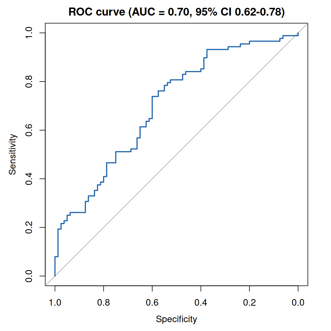
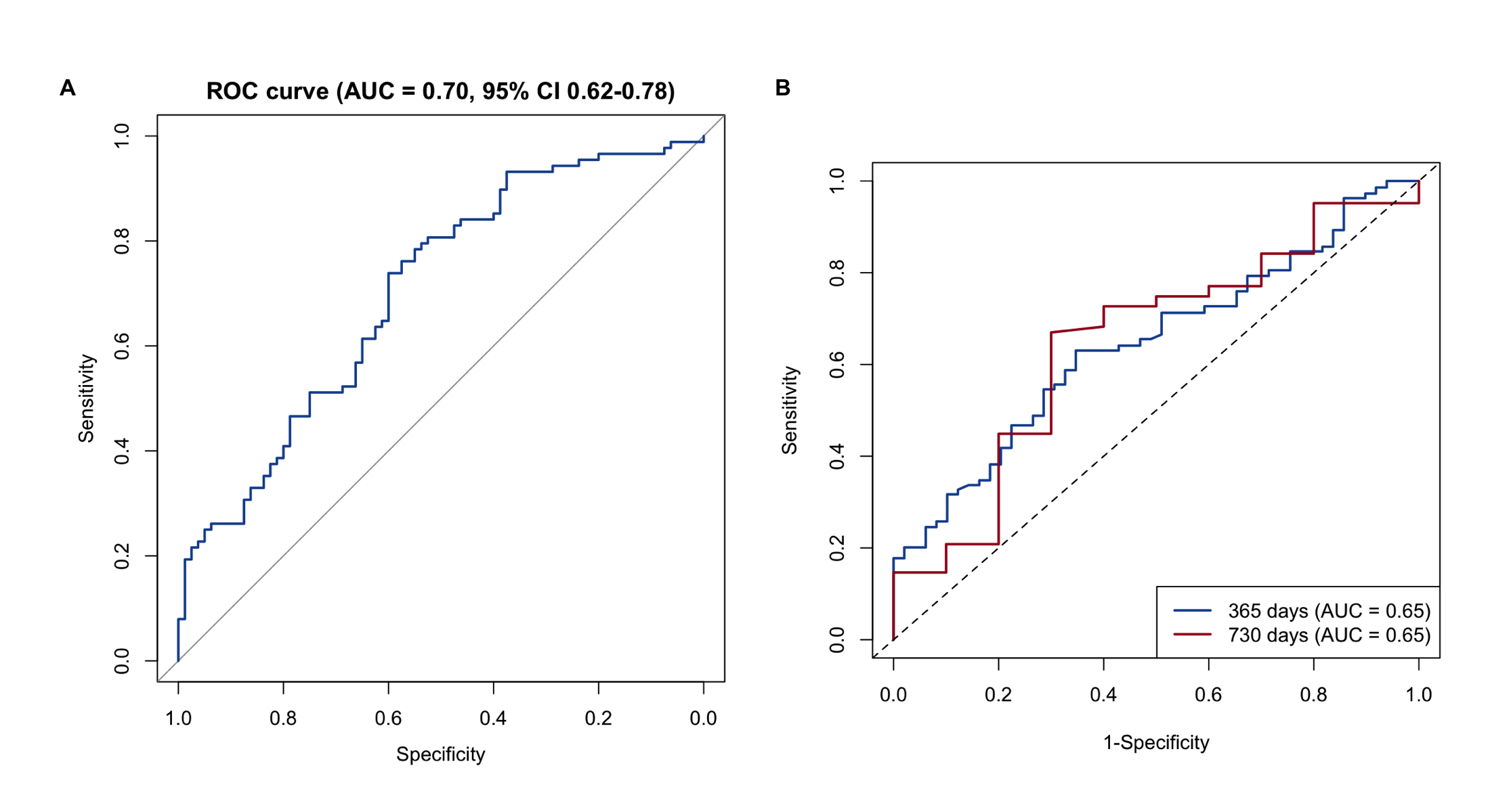
The AUC of 0.70 indicates acceptable discrimination of 1-year mortality. The bootstrap confidence interval quantifies the sampling uncertainty of the estimate.
2. Comparing Two Models with the DeLong Test
A common question is whether the extra covariates of a full model actually improve discrimination over a simpler model. The DeLong test compares paired ROC curves without resampling.
roc_simple <- roc(lung2$y1y, fitted(m_simple), quiet = TRUE)
roc_test <- roc.test(roc_full, roc_simple, method = "delong")

plot(roc_full, col = "#2166AC", lwd = 2,
     main = sprintf("Full vs simple model (DeLong p = %.3f)", roc_test$p.value))
plot(roc_simple, col = "#B2182B", lwd = 2, lty = 2, add = TRUE)
legend("bottomright",
       legend = c(sprintf("Full model (AUC = %.2f)", auc(roc_full)),
                  sprintf("ECOG only (AUC = %.2f)", auc(roc_simple))),
       col = c("#2166AC", "#B2182B"), lwd = 2, lty = c(1, 2))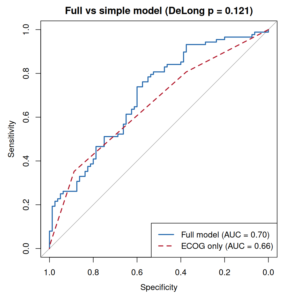
Here the difference is not statistically significant (p = 0.121), which cautions against claiming added value from the extra covariates in this small data set.
3. Optimal Cutoff Selection
best <- coords(roc_full, x = "best", input = "threshold",
               best.method = "youden", ret = c("threshold", "specificity", "sensitivity"))
print(best)
threshold specificity sensitivity
1 0.4555072 0.6 0.7386364plot(roc_full, col = "#2166AC", lwd = 2, print.thres = "best",
print.thres.best.method = "youden",
main = "ROC curve with Youden-optimal threshold")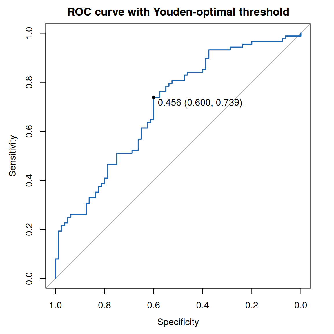
The Youden index picks the threshold maximizing sensitivity + specificity − 1. Note that a single “optimal” cutoff is context-dependent: clinical consequences (costs of false positives vs false negatives) should guide the choice, e.g. via decision curve analysis.
4. Publication-Style ROC with plotROC
longdf <- melt_roc(lung2, d = "y1y", m = c("risk_full", "risk_ecog")) |>
  mutate(name = ifelse(name == "risk_full", "Full model", "ECOG only"))

# Named vectors: match colors/labels to models regardless of level ordering
model_colors <- c("Full model" = "#2166AC", "ECOG only" = "#B2182B")
model_labels <- c("Full model" = paste0("Full model (AUC = ", round(auc(roc_full), 2), ")"),
                  "ECOG only"  = paste0("ECOG only (AUC = ", round(auc(roc_simple), 2), ")"))
ggplot(longdf, aes(d = D, m = M, color = name)) +
  geom_roc(labels = FALSE, linewidth = 1) +
  style_roc(theme = theme_grey()) +
  scale_color_manual(values = model_colors, labels = model_labels, name = "Model") +
  labs(title = "ROC curves built with ggplot2")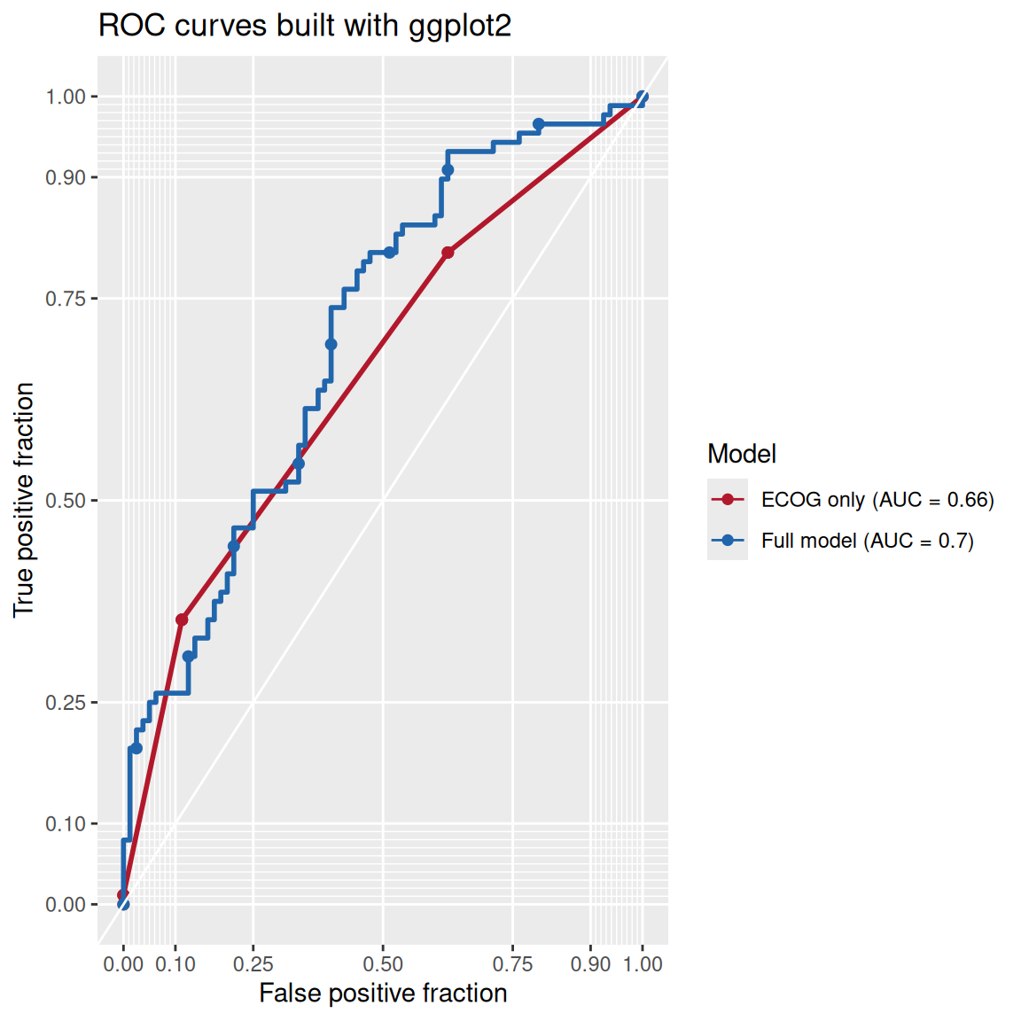
melt_roc() converts the data to long format and geom_roc() draws the curves; the AUCs are computed with pROC and reported in the legend.
5. Time-Dependent ROC with timeROC
For survival endpoints, standard ROC ignores censoring. Time-dependent ROC evaluates discrimination at a fixed horizon, e.g. 1-year and 2-year mortality predicted by the Cox risk score [3].
tr <- timeROC(T = as.numeric(lung2$time),
              delta = ifelse(lung2$status == 2, 1, 0),  # 1 = event, 0 = censored
              marker = lung2$risk_score, cause = 1,
              weighting = "marginal",
              times = c(365, 730), ROC = TRUE, iid = TRUE)

plot(tr, time = 365, col = "#2166AC", lwd = 2,
     title = "Time-dependent ROC of the Cox risk score")
plot(tr, time = 730, col = "#B2182B", lwd = 2, add = TRUE)
legend("bottomright",
       legend = sprintf("%d days (AUC = %.2f)", c(365, 730), tr$AUC),
       col = c("#2166AC", "#B2182B"), lwd = 2)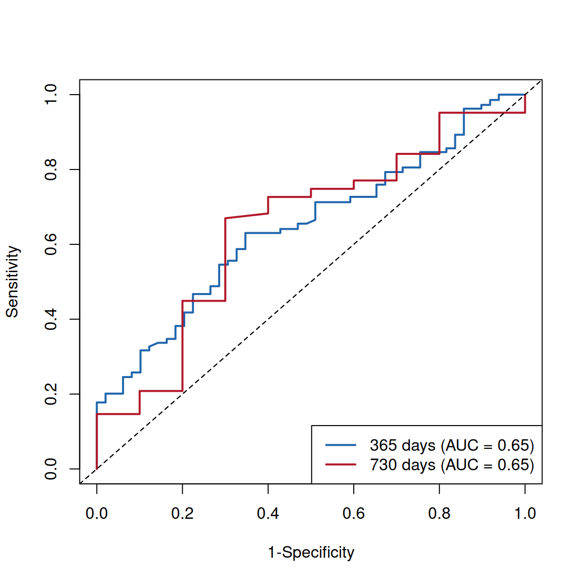
Important details: delta uses the coding 0 = censored and 1 = event of interest (this is not the raw status coding of lung, where 1 means censored); the risk score is a continuous marker derived from the Cox model. Confidence intervals of the time-dependent AUC are available through confint(tr) because iid = TRUE was requested.
Application
Time-dependent ROC curves are widely used in oncology prognostic-model papers to report discrimination at clinically meaningful horizons (1, 3, 5 years), often next to calibration curves and decision curve analysis. The panel below mirrors that publication layout with this tutorial’s outputs: (A) standard ROC of the binary model and (B) time-dependent ROC at fixed horizons.
Reference
[1] Loprinzi CL, Laurie JA, Wieand HS, et al. Prospective evaluation of prognostic variables from patient-completed questionnaires. North Central Cancer Treatment Group. J Clin Oncol. 1994;12(3):601-607. doi:10.1200/JCO.1994.12.3.601
[2] Robin X, Turck N, Hainard A, et al. pROC: an open-source package for R and S+ to analyze and compare ROC curves. BMC Bioinformatics. 2011;12:77. doi:10.1186/1471-2105-12-77
[3] Blanche P, Dartigues JF, Jacqmin-Gadda H. Estimating and comparing time-dependent areas under receiver operating characteristic curves for censored event times with competing risks. Stat Med. 2013;32(30):5381-5397. doi:10.1002/sim.5958
[4] Sachs MC. plotROC: A Tool for Plotting ROC Curves. J Stat Softw Code Snippets. 2017;79(2):1-12. doi:10.18637/jss.v079.c02