# Installing packages
if (!requireNamespace("pathview", quietly = TRUE)) {
  remotes::install_github("datapplab/pathview")
}
if (!requireNamespace("dbplyr", quietly = TRUE)) {
  install.packages("dbplyr")
}

# Load packages
library(pathview)
library(dbplyr)KEGG Pathway Plot
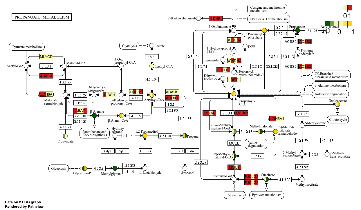
Example
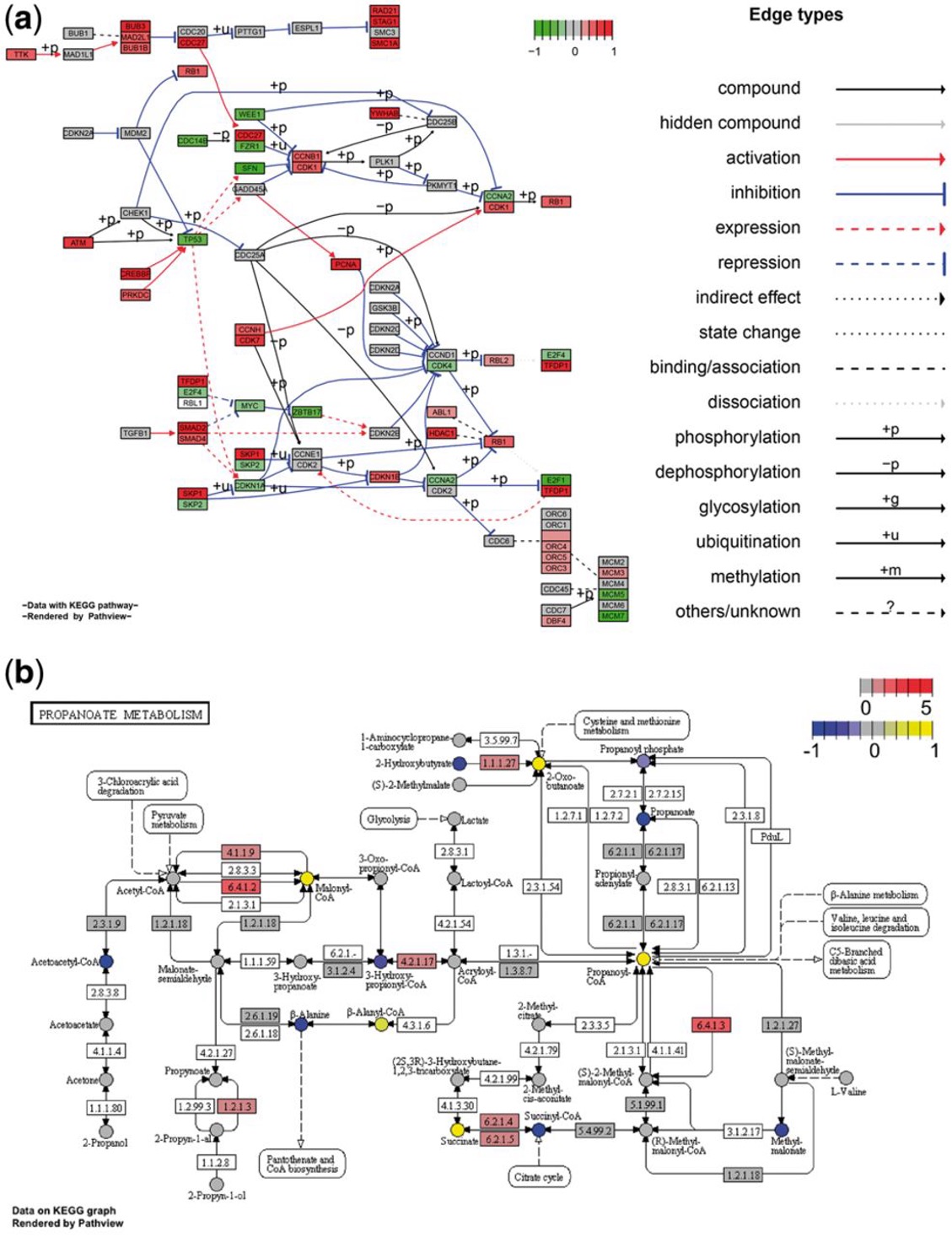
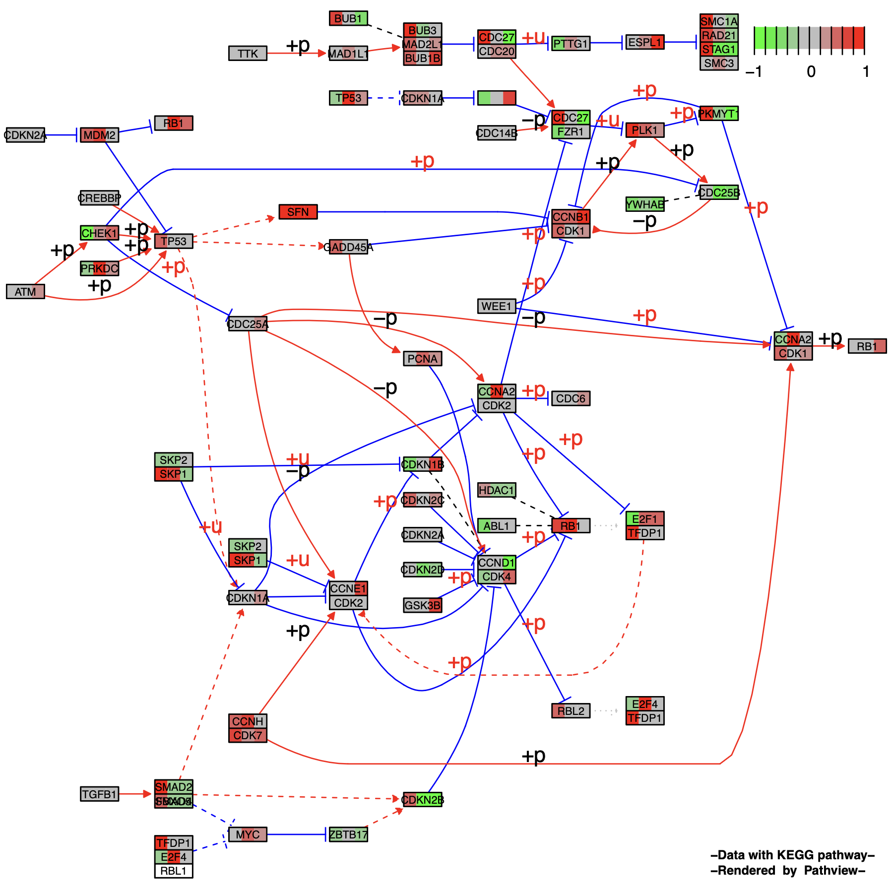
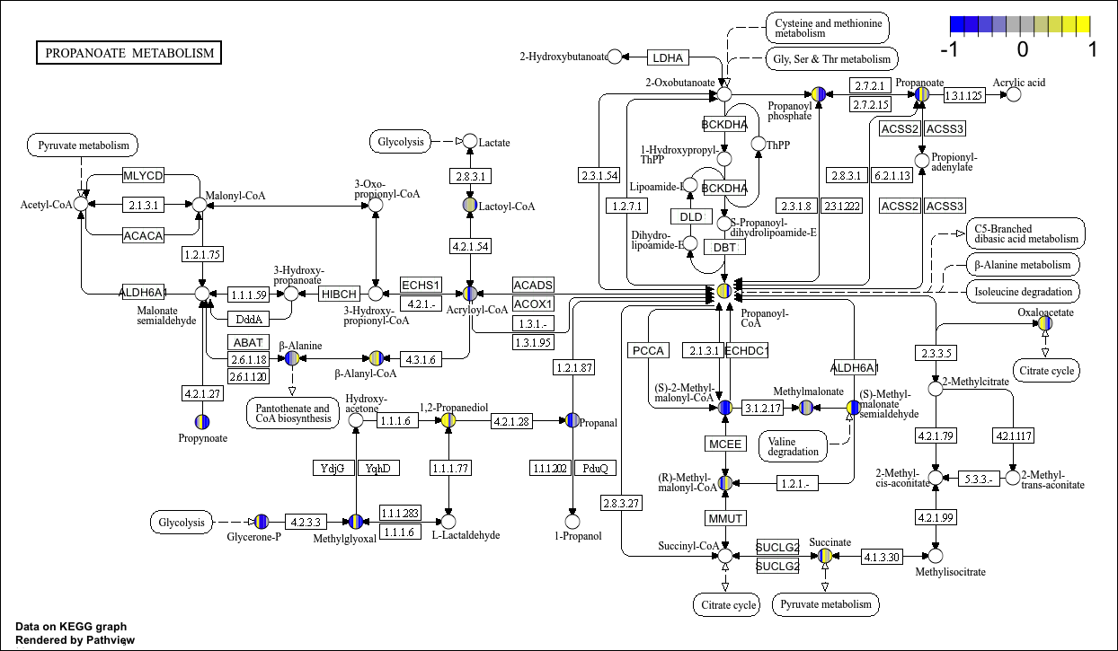
- Graphviz view showing a classical signaling pathway (hsa04110 Cell cycle) containing gene data; (b) KEGG view showing a metabolic pathway (hsa00640 Propanoate metabolism) containing discrete gene data and continuous metabolite data.
The images and R packages are from the article by Luo et al. [1]
Setup
System Requirements: Cross-platform (Linux/MacOS/Windows)
Programming language: R
Dependent packages:
pathview,dbplyr
sessioninfo::session_info("attached")─ Session info ───────────────────────────────────────────────────────────────
setting value
version R version 4.6.0 (2026-04-24)
os Ubuntu 24.04.4 LTS
system x86_64, linux-gnu
ui X11
language (EN)
collate C.UTF-8
ctype C.UTF-8
tz UTC
date 2026-05-09
pandoc 3.1.3 @ /usr/bin/ (via rmarkdown)
quarto 1.9.37 @ /usr/local/bin/quarto
─ Packages ───────────────────────────────────────────────────────────────────
package * version date (UTC) lib source
dbplyr * 2.5.2 2026-02-13 [1] RSPM
pathview * 1.47.1 2026-05-04 [1] Github (datapplab/pathview@1f17eb7)
[1] /home/runner/work/_temp/Library
[2] /opt/R/4.6.0/lib/R/site-library
[3] /opt/R/4.6.0/lib/R/library
* ── Packages attached to the search path.
──────────────────────────────────────────────────────────────────────────────Data Preparation
The example data is a gene expression matrix: the ENTREZ IDs of behavioral genes are listed as sample names, and the expression data is normalized. This can be any numerical data type, such as fold change, p-value, etc., depending on your needs.
data("gse16873.d")
head(gse16873.d)
DCIS_1 DCIS_2 DCIS_3 DCIS_4 DCIS_5
10000 -0.30764480 -0.14722769 -0.023784808 -0.07056193 -0.001323087
10001 0.41586805 -0.33477259 -0.513136907 -0.16653712 0.111122223
10002 0.19854925 0.03789588 0.341865341 -0.08527420 0.767559264
10003 -0.23155297 -0.09659311 -0.104727283 -0.04801404 -0.208056443
100048912 -0.04490724 -0.05203146 0.036390376 0.04807823 0.027205816
10004 -0.08756237 -0.05027725 0.001821133 0.03023835 0.008034394
DCIS_6
10000 -0.15026813
10001 0.13400734
10002 0.15828609
10003 0.03344448
100048912 0.05444739
10004 -0.06860749gene_data <- as.data.frame(gse16873.d)
head(gene_data) DCIS_1 DCIS_2 DCIS_3 DCIS_4 DCIS_5
10000 -0.30764480 -0.14722769 -0.023784808 -0.07056193 -0.001323087
10001 0.41586805 -0.33477259 -0.513136907 -0.16653712 0.111122223
10002 0.19854925 0.03789588 0.341865341 -0.08527420 0.767559264
10003 -0.23155297 -0.09659311 -0.104727283 -0.04801404 -0.208056443
100048912 -0.04490724 -0.05203146 0.036390376 0.04807823 0.027205816
10004 -0.08756237 -0.05027725 0.001821133 0.03023835 0.008034394
DCIS_6
10000 -0.15026813
10001 0.13400734
10002 0.15828609
10003 0.03344448
100048912 0.05444739
10004 -0.06860749Visualization
1. Basic Plot
Observe the cell cycle signaling pathway diagram of a single sample (DCIS_1) (KEGG ID: 04110).
1.1 KEGG View
When kegg.native = TRUE is set, the output pathway diagram is drawn based on the original KEGG view. The output image is automatically saved in the current directory.
p1 <- pathview(gene.data = gse16873.d[, 1], # Input gene matrix
               pathway.id = "04110", # Pathway ID
               species = "hsa", # Species: Human
               out.suffix = "gse16873_KEGG", # Output file suffix
               kegg.native = T, # Output in original KEGG view
               same.layer = T # Drawing a single layer
               )
p1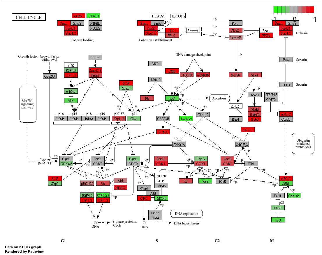
To better understand kegg.native = TRUE, let’s compare it with the Cell cycle pathway map on the KEGG official website (https://www.kegg.jp/pathway/map04110)
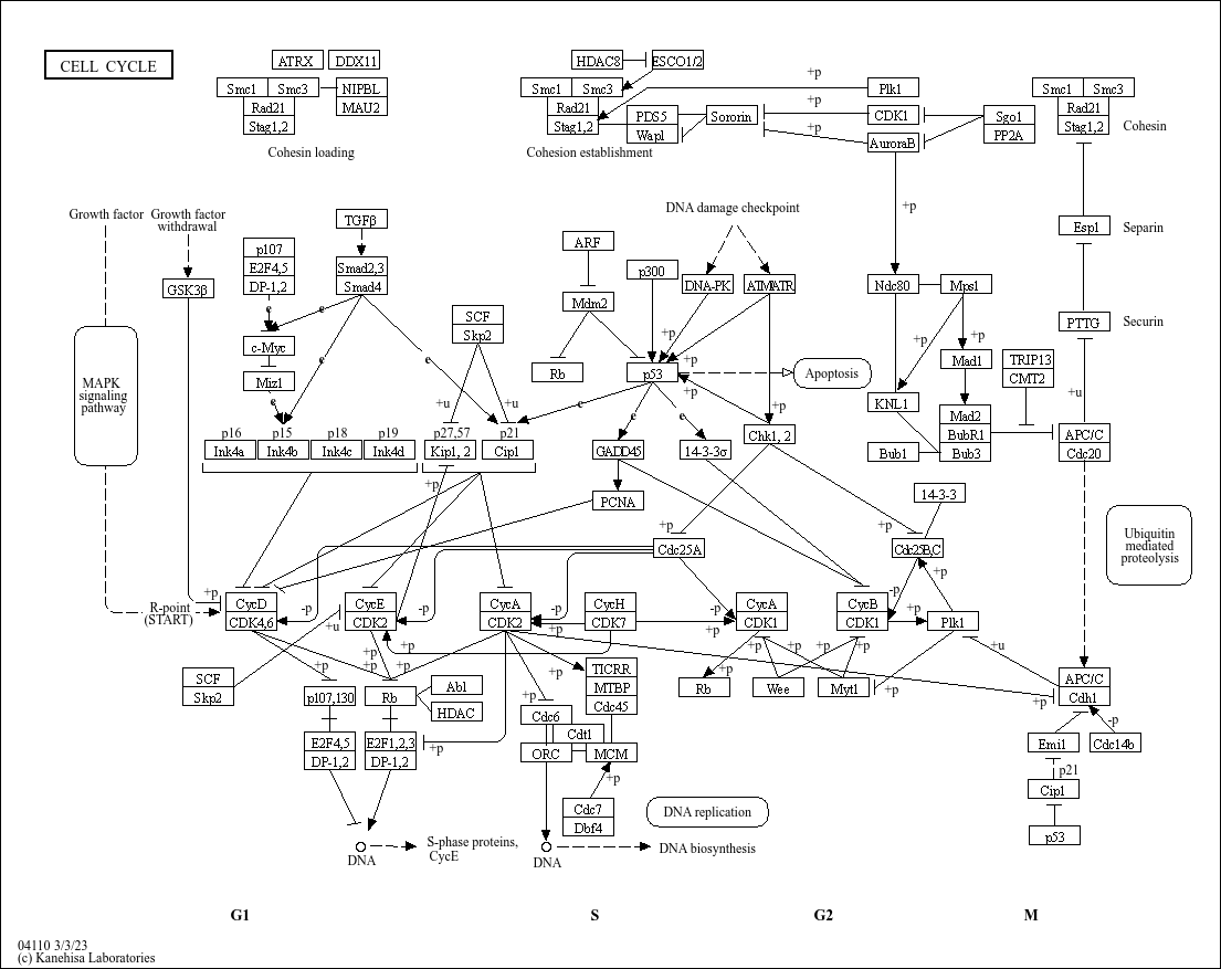
It’s easy to see that the resulting graph we’ve output is based on the pathway diagram provided on the official website, visualizing the differential expression of pathway genes across the study samples. However, when kegg.native = FALSE is used instead, the Graphviz engine is used to generate the graph, and the output is a vector graph in PDF format, which will be discussed later.
Next, let’s examine the structure of the pathview function’s output, p1 . It’s a list of length 2, containing the data we need for our graph.
Tip
plot.data.gene (data.frame): stores the gene data used for plotting.plot.data.cpd (data.frame): stores the compound data used for plotting.kegg.names: the KEGG-formatted IDs of the genes/compounds mapped to the node (i.e., Entrez Gene IDs or KEGG Compound Accessions).labels: the names of the genes/compounds mapped to the node.all.mapped: the IDs of all genes/compounds mapped to the node.type: the node type (“gene”, “enzyme”, “compound”, “homolog”)x: the x-coordinate in the original KEGG pathway graph.y: the y-coordinate in the original KEGG pathway graph.width: the width of the node in the original KEGG pathway graph.height: the height of the node in the original KEGG pathway graph.mol.data: Data for the gene/compound mapped to the node (corresponding to the input data gene.data)mol.data: Color codes for the gene/compound mapped to the node
1.2 Graphviz View
After introducing the output of images in KEGG native form (kegg.native = TRUE), let’s take a look at the image format of the graph output using Graphviz (kegg.native = FALSE).
p2 <- pathview(gene.data = gse16873.d[, 1],
               pathway.id = "04110",
               species = "hsa",
               out.suffix = "gse16873_Graph",
               kegg.native = F ,# Output in Graphviz format
               same.layer = T # Drawing a single layer
               )
p2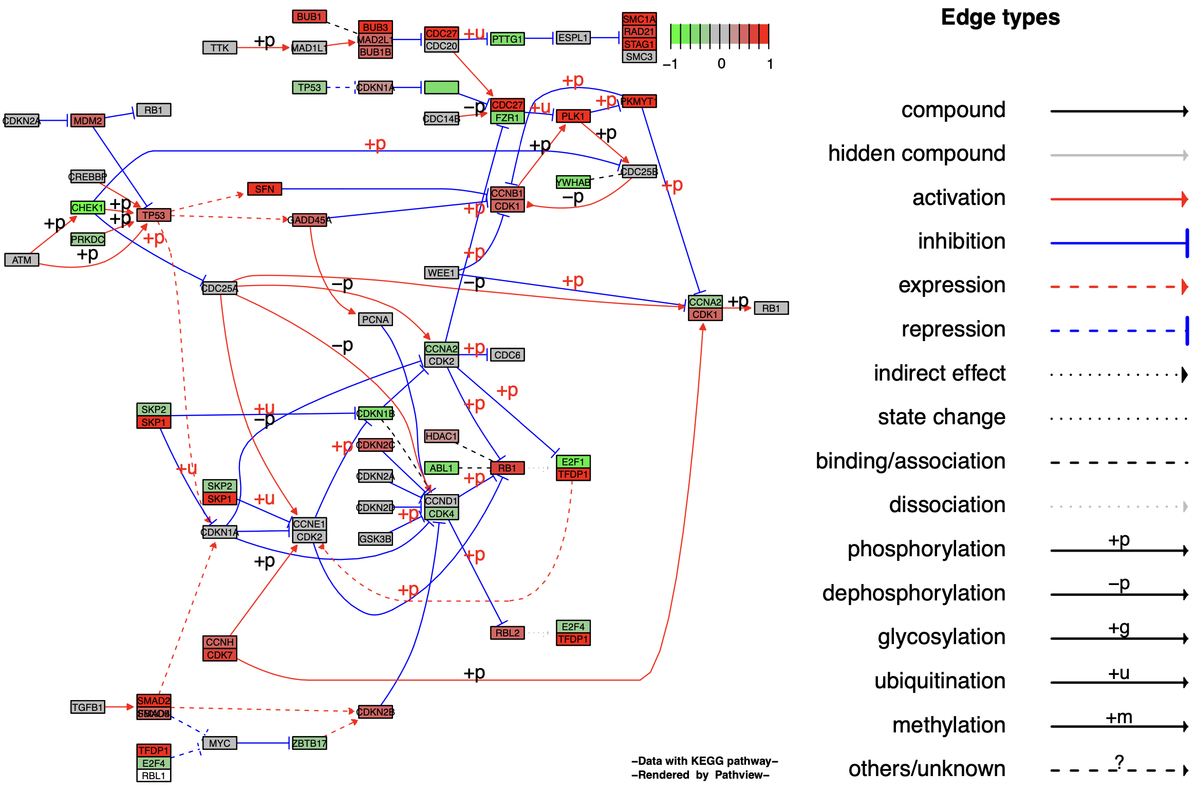
The KEGG native format preserves all pathway metadata, including spatial and temporal information, tissue/cell types, inputs, outputs, and connections, which is crucial for readability and interpretation of pathway biology. The Graphviz view, however, is a vector PDF format, providing greater control over node and edge properties and a better visualization of pathway topology, allowing for further enhancement using, for example, Adobe illustrations.
In pathway diagrams exported in Graphviz format, the same.layer parameter has a different meaning than in the KEGG native format. It now describes the layer relationship between the legend and the pathway diagram. When same.layer = TRUE, the legend and pathway diagram appear on the same layer, and the legend only describes edge types, omitting node types.
When same.layer = FALSE, the legend and pathway diagram appear on separate layers, describing both edge and node types.
p3 <- pathview(gene.data = gse16873.d[, 1],
               pathway.id = "04110",
               species = "hsa",
               out.suffix = "gse16873_Graph",
               kegg.native = F ,# Output in Graphviz format
               same.layer = T # Drawing a single layer
               )
p3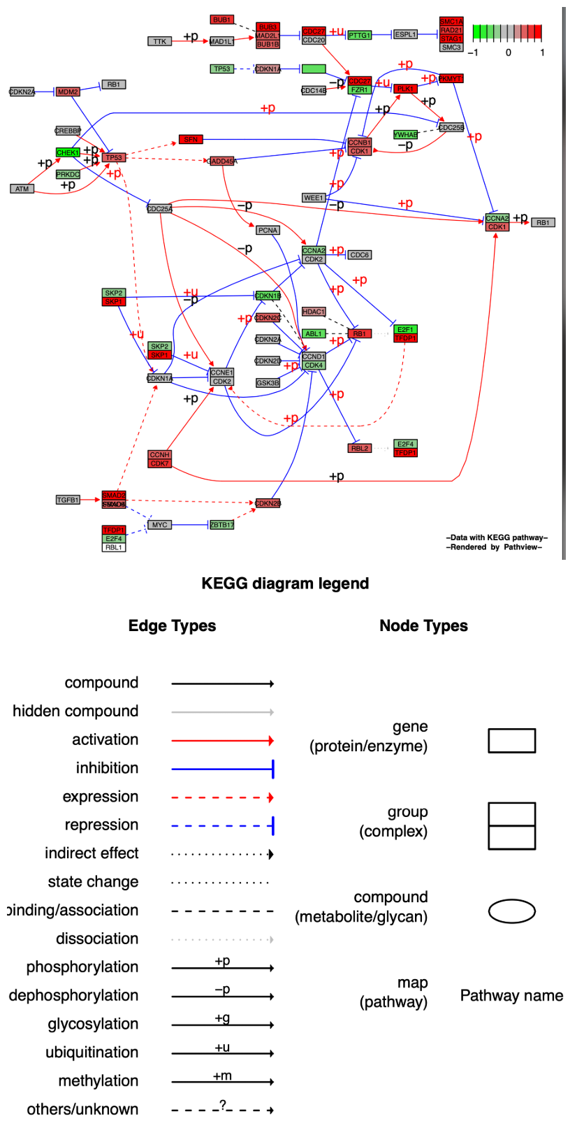
2. Graphics Adjustment
Considering that many parameters that change the graphic style only take effect when kegg.native = FALSE, we will also draw based on this in most cases.
2.1 Node style adjustment
p4 <- pathview(gene.data = gse16873.d[, 1],
               pathway.id = "04110",
               species = "hsa",
               out.suffix = "gse16873_node",
               kegg.native = F ,
               same.layer = F ,
               low = '#4575B4',
               mid = '#F7F7BD',
               high = '#D73027',
               cex = 0.5 , # Font size
               afactor = 1.6 , # Node size
               limit = list( gene = 2 ) # Legend upper and lower limits
               )
p4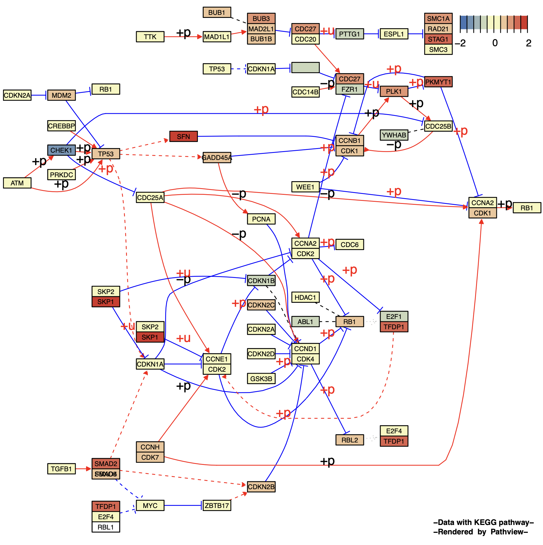
2.2 Node splitting and expansion
Splitting a node group into individual nodes can be controlled by setting the split.group parameter. Setting expand.node can expand a multi-gene node into a single gene.
Split a node group (split.group = TRUE):
p5 <- pathview(gene.data = gse16873.d[, 1],
               pathway.id = "04110",
               species = "hsa",
               out.suffix = "gse16873_split",
               kegg.native = F ,
               same.layer = F ,
               split.group = T # TRUE
               )

p5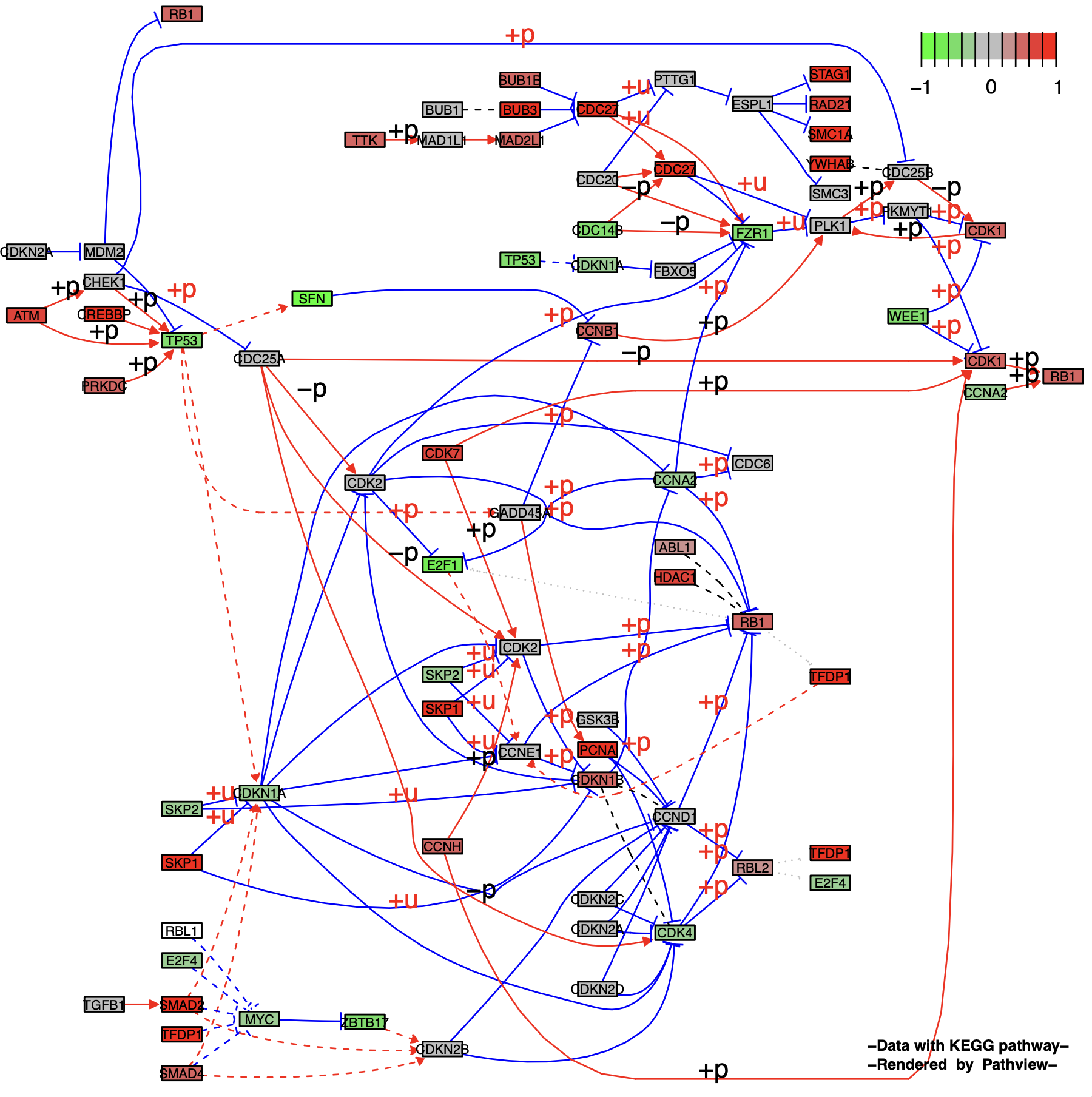
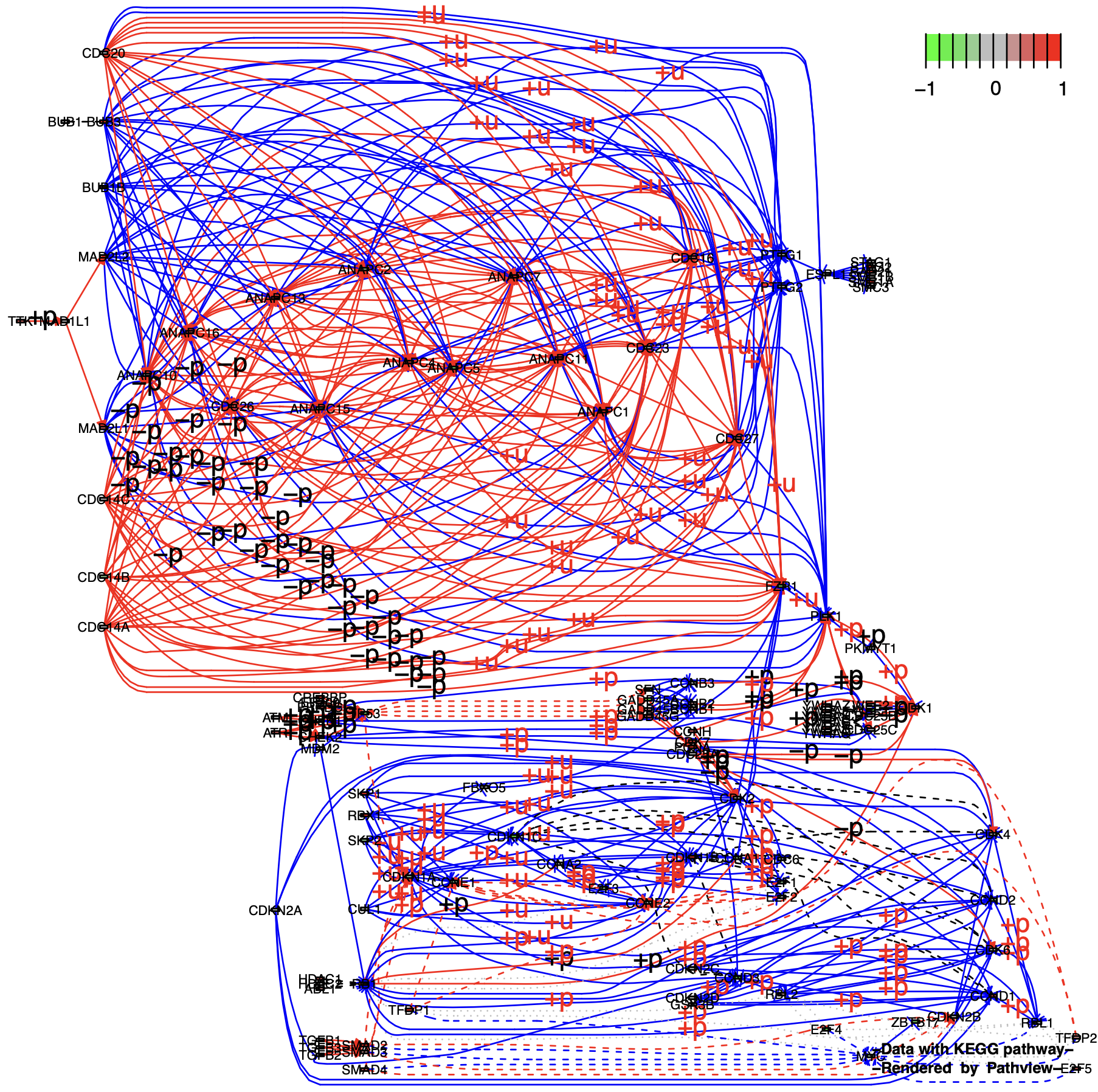
Multi-gene nodes are expanded to single genes: (split.group = TRUE & expand.node = TRUE):
p6 <- pathview(gene.data = gse16873.d[, 1],
               pathway.id = "04110",
               species = "hsa",
               out.suffix = "gse16873_expand",
               kegg.native = F ,
               same.layer = F ,
               split.group = T,
               expand.node = T # TRUE
               )

unique(p6$plot.data.gene$kegg.names) %>% length()
# [1] 88
unique(p7$plot.data.gene$kegg.names) %>% length()
# [1] 158

# The extra nodes are the extensions of the original multi-gene nodes
setdiff(unique(B),intersect(A,B))
Then we found that the lines became so complicated that the nodes and relationships between nodes that we were focusing on were lost.
2.3 Multiple groups of samples
The above example plots the pathway diagram for a single sample. To compare pathway changes across two or more samples, set multi.state = TRUE. This allows you to combine data from multiple samples into a single pathway diagram. In this case, each node will be split into multiple segments, one for each sample.
p8 <- pathview(gene.data = gse16873.d[, 1:3], # Multiple groups of samples
               pathway.id = "04110",
               species = "hsa",
               out.suffix = "gse16873_samples",
               kegg.native = F ,
               same.layer = F ,
               multi.state = T #
               )
The effect is that the node is divided into multiple segments corresponding to the number of samples, and one sample corresponds to one color block.
2.4 Pathway diagram of the compound
Compound data
Previously, we only introduced pathway visualization of gene data. If you are only working with compound data, it is actually the same as gene data. You only need to change gene.data to cpd.data.
# Simulate compound data for 6 samples
data("cpd.simtypes")
cpd_data <- sim.mol.data(mol.type="cpd", nmol=3000)
cpd_data2 <- matrix(sample(cpd_data,18000,replace = T), ncol = 6)
rownames(cpd_data2) = names(cpd_data)
colnames(cpd_data2) = colnames(gene_data)
head(cpd_data2)
KEGG View
p9 <- pathview(cpd.data = cpd_data2, # Compound data
               pathway.id = "00640", #
               species = "hsa",
               out.suffix = "gse16873_KEGG_cpd",
               kegg.native = T , # KEGG View
               same.layer = F
) 
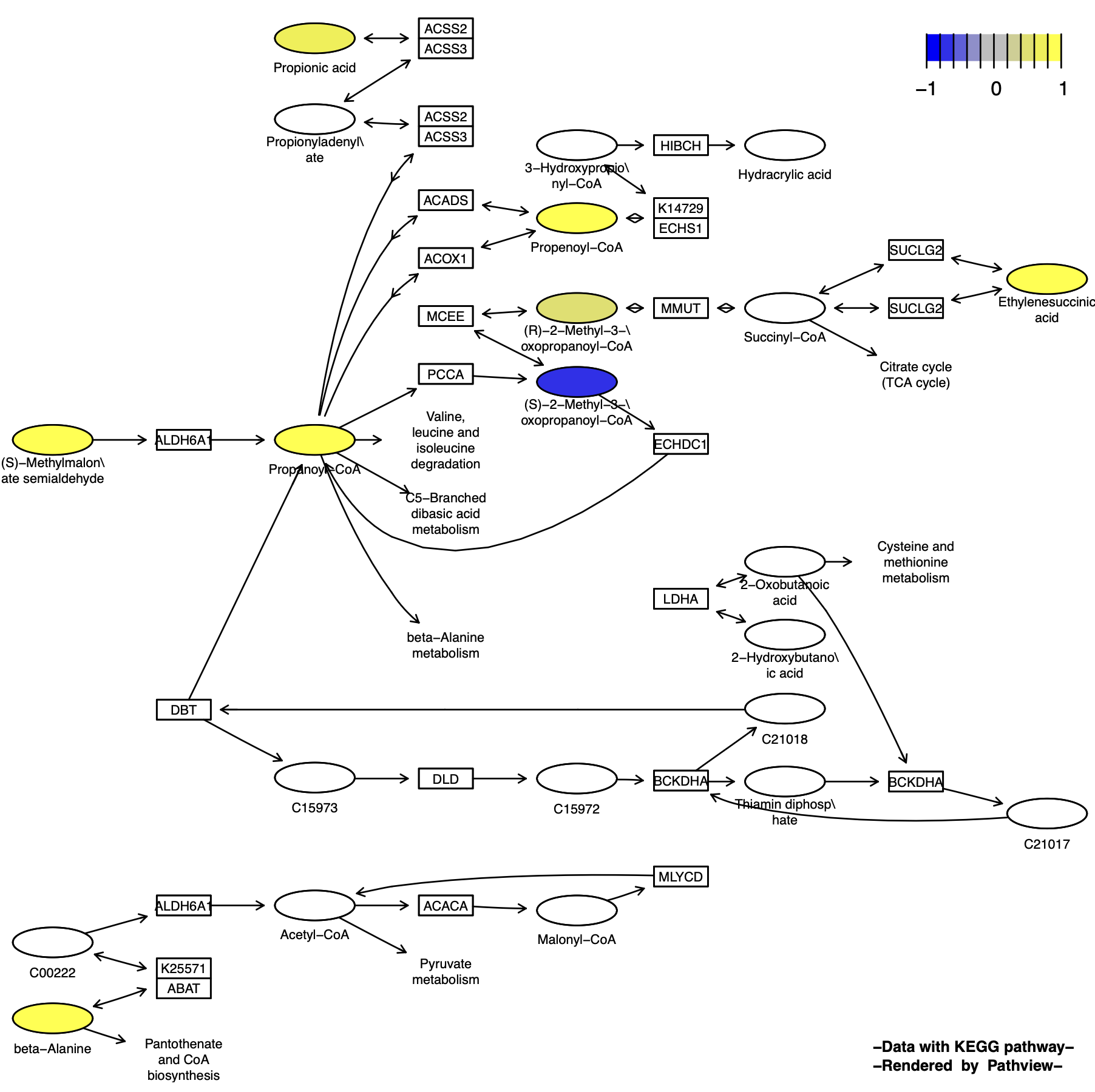
Graphviz View
p10 <- pathview(cpd.data = cpd_data, # Compound data
               pathway.id = "00640",
               species = "hsa",
               out.suffix = "gse16873_Graphviz_cpd",
               kegg.native = F , # Graphviz View"
               same.layer = F  ,
               cpd.lab.offset = -1.0 # Compound label position
) 
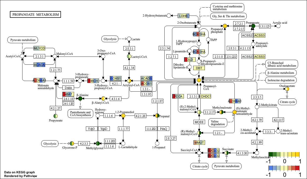
Compound and gene data据
Next we illustrate the case of plotting gene and compound data simultaneously:
KEGG View
p11 <- pathview(gene.data = gene_data[,1:4], # Gene data
               cpd.data = cpd_data2[,1:2], # Compound data
               pathway.id = "00640",
               species = "hsa",
               out.suffix = "gse16873_KEGG_gene_cpd",
               kegg.native = T , # KEGG View
               same.layer = F  ,
               cpd.lab.offset = -1.0 ,
               key.pos = 'bottomright',
               match.data = F, # Not match sample
               multi.state = T ,
               bins = list(gene = 8, cpd = 8), # Change the number of legend color blocks
               low = list(gene = "#6495ED", cpd = "#006400"),
               mid = list(gene = "#F7F7BD", cpd = "#F7F7BD"),
               high = list(gene = "#D73027", cpd ="#FFD700")
) 
Graphviz View
p12 <- pathview(gene.data = gene_data[,1:4], # Gene data
               cpd.data = cpd_data2[,1:2], # Compound data
               pathway.id = "00640",
               species = "hsa",
               out.suffix = "gse16873_Graphviz_gene_cpd",
               kegg.native = F , # Graphviz View
               same.layer = F  ,
               cpd.lab.offset = -1.0 ,
               key.pos = 'topright',
               match.data = F, # Not match sample
               multi.state = T ,
               bins = list(gene = 10, cpd = 10), # Change the number of legend color blocks
               low = list(gene = "#6495ED", cpd = "#006400"),
               mid = list(gene = "#F7F7BD", cpd = "#F7F7BD"),
               high = list(gene = "#D73027", cpd ="#FFD700")
) 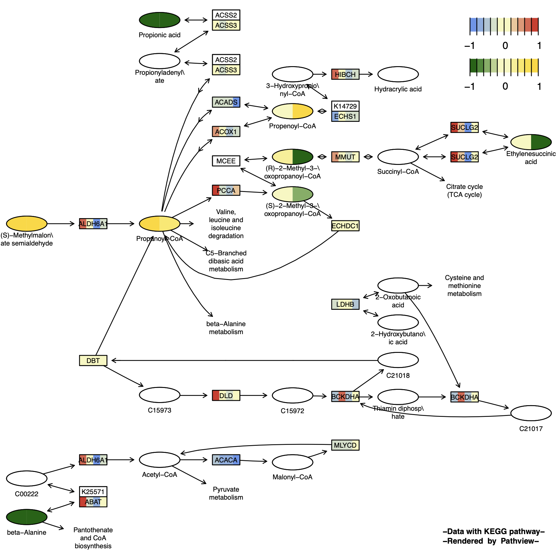
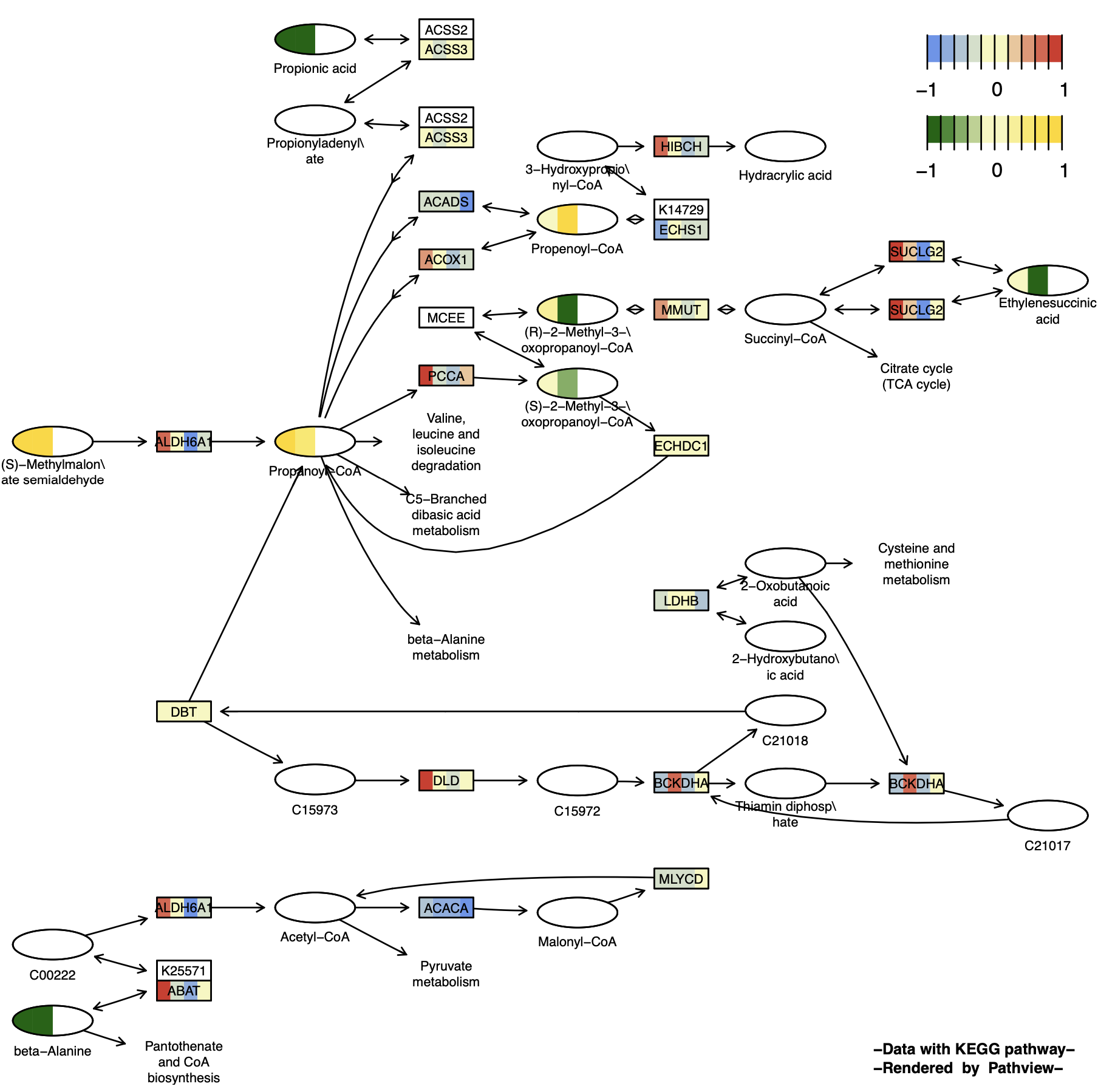
When the gene and cpd data have different sample numbers, the parameter match.data = FALSE should be set. If match.data = TRUE is set, the data with fewer samples will generate a column of NAs to match the sample numbers. NA data is transparent by default, but the color can be set using na.col.
p13 <- pathview(gene.data = gene_data[,1:4],
               cpd.data = cpd_data2[,1:2],
               pathway.id = "00640",
               species = "hsa",
               out.suffix = "gse16873_Graphviz_gene_cpd_match",
               kegg.native = F , # Graphviz View
               same.layer = F  ,
               cpd.lab.offset = -1.0 ,
               key.pos = 'topright',
               match.data = T, # Matching number of samples: Add 2 columns of NA for cpd
               multi.state = T ,
               bins = list(gene = 10, cpd = 10),
               na.col = 'transparent' , # NA data color setting
               low = list(gene = "#6495ED", cpd = "#006400"),
               mid = list(gene = "#F7F7BD", cpd = "#F7F7BD"),
               high = list(gene = "#D73027", cpd ="#FFD700")
               )
You can see that only half of the compound node is colored because the other half is NA and is transparent and colorless by default.
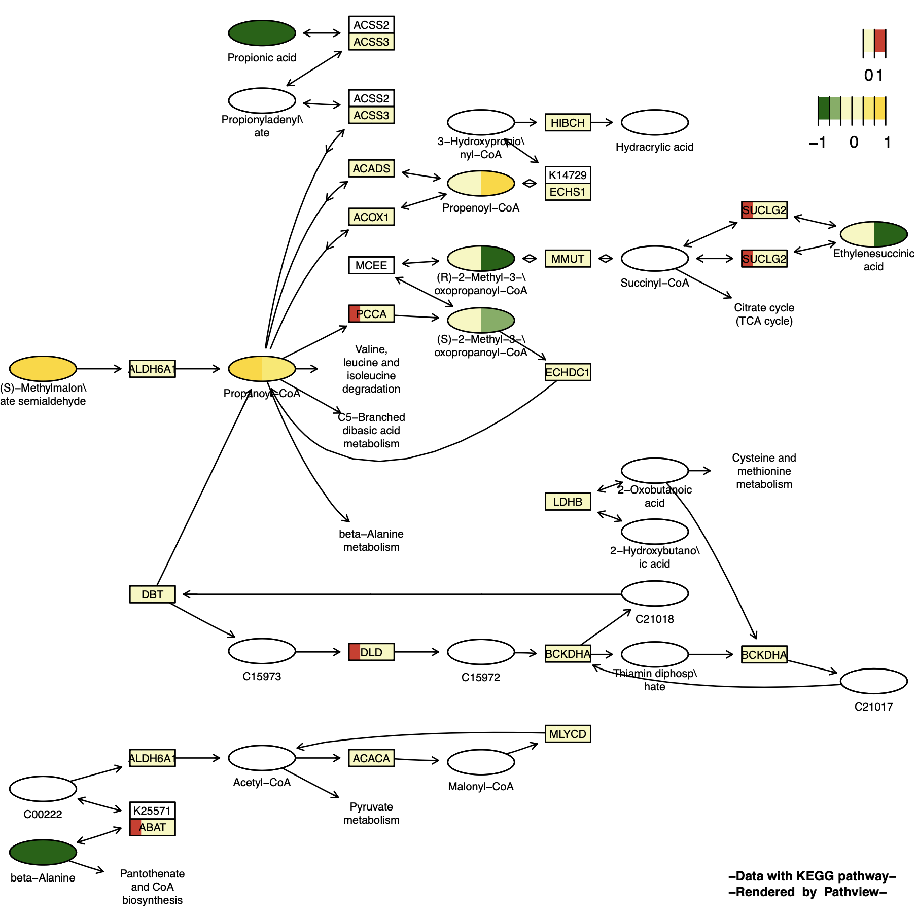
2.5 Discrete data
If our input data is not a continuous variable like in the example above, but rather a categorical variable such as high/low (which can be replaced by 1/0) or the names of significantly differentially expressed genes, we need to set the discrete parameter to plot a pathway view of the discrete variable.
Here, we treat the gene data as a discrete variable of 1/0 and the compound as a continuous variable.
# Obtaining genetic data (discrete variables)
data("gse16873.d")
gene_data <- gse16873.d
colnames(gene_data)
gene_data2 <- apply(gene_data, 2, function(x){
  ifelse(x > mean(x), 1 , 0 )
}) %>% as.data.frame()
str(gene_data2)
p14 <- pathview(gene.data = gene_data2[,1:4], # Discrete variables
cpd.data = cpd_data2[,1:2], # Continuous variables
pathway.id = "00640",
species = "hsa",
out.suffix = "gse16873_KEGG_gene_cpd_discrete",
kegg.native = T , # KEGG View
same.layer = F ,
cpd.lab.offset = -1.0 ,
key.pos = 'topright',
match.data = F,
multi.state = T ,
bins = list(gene = 1, cpd = 6),
low = list(gene = "#F7F7BD", cpd = "#006400"),
mid = list(gene = "#F7F7BD", cpd = "#F7F7BD"),
high = list(gene = "#D73027", cpd ="#FFD700"),
discrete = list(gene = T, cpd = F) ,# Discrete data is T
limit = list(gene = 1, cpd = c(-1,1)) ,
both.dirs = list(gene = F, cpd = T) # gene is one-way data
) 
p15 <- pathview(gene.data = gene_data[,1:4], # Discrete variables
               cpd.data = cpd_data2[,1:2], # Continuous variables
               pathway.id = "00640",
               species = "hsa",
               out.suffix = "gse16873_Graphviz_gene_cpd_discrete",
               kegg.native = F , # Graphviz View
               same.layer = F  ,
               cpd.lab.offset = -1.0 ,
               key.pos = 'topright',
               match.data = F,
               multi.state = T ,
               bins = list(gene = 1, cpd = 6),
               low = list(gene = "#F7F7BD", cpd = "#006400"),
               mid = list(gene = "#F7F7BD", cpd = "#F7F7BD"),
               high = list(gene = "#D73027", cpd ="#FFD700"),
               discrete = list(gene = T, cpd = F) ,# Discrete data is T
               limit = list(gene = 1, cpd = c(-1,1)),
               both.dirs = list(gene = F, cpd = T) # gene.data is one-way data
) 
Application
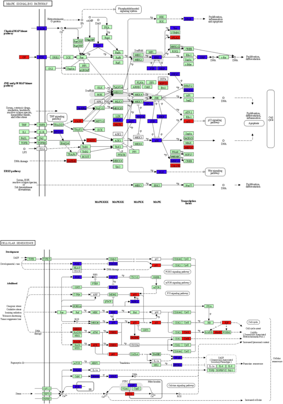
This figure illustrates key KEGG pathways: MAPK signaling pathway and cellular senescence signaling pathway. The red nodes represent upregulated DEGs in cingulin b-MO mutants, the green marked node represents downregulated DEGs in cingulin b-MO mutants, and the blue marked node represents overlapping targets between Control-MO and cingulin b-MO embryos. The analysis is conducted from three independent experiments in different groups, and each group has 30 embryos. [2]
Reference
[1] Luo, W., & Brouwer, C. (2013). Pathview: an R/Bioconductor package for pathway-based data integration and visualization. Bioinformatics (Oxford, England), 29(14), 1830–1831. https://doi.org/10.1093/bioinformatics/btt285IF: 4.4 B3.
[2] Lu Y, Tang D, Zheng Z, et al. Cingulin b Is Required for Zebrafish Lateral Line Development Through Regulation of Mitogen-Activated Protein Kinase and Cellular Senescence Signaling Pathways. Front Mol Neurosci. 2022;15:844668. Published 2022 May 5. doi:10.3389/fnmol.2022.844668.