Paired Before-After Plot (Python)

Authors

[Contributors] Codex (GPT-5) — AI-generated, independently AI-reviewed;

Modified

2026-11-05

🤖 AI Skill — Download the Bizard unified skill for your AI assistant ⬇️ Download Skill ZIP

🔌 MCP Server — Let AI agents (Claude Code, Cursor, …) query Bizard live: claude mcp add bizard -- npx @openbiox/bizard-mcp — or the free hosted instance (no install, faster from mainland China): claude mcp add --transport http bizard http://biotree.top:38123/bizard-mcp/mcp 📖 MCP Docs

📖 Cite Bizard — if Bizard helps your research, please cite: Li, K., Zheng, H., Huang, K., et al. (2026). Bizard: A Community-Driven Platform for Accelerating and Enhancing Biomedical Data Visualization. iMetaMed, e70038. 🔗 DOI / BibTeX

The Python counterpart of Paired Plot — a paired before-after plot draws one line, arrow, or dumbbell per subject between the two time points, keeping the pairing visible. It is the honest alternative to two side-by-side boxplots for paired designs: baseline vs follow-up biomarker, pre vs post treatment lesion size (RECIST workflows), or within-patient case-control measurements.

matplotlib draws all three variants; scipy.stats.ttest_rel annotates the paired t-test [1]. The central design rule: the subject is the unit of analysis, so every subject must remain traceable in the figure — aggregates hide heterogeneity such as “half the cohort shrinks, half grows, mean unchanged”.

This tutorial covers three workflows:

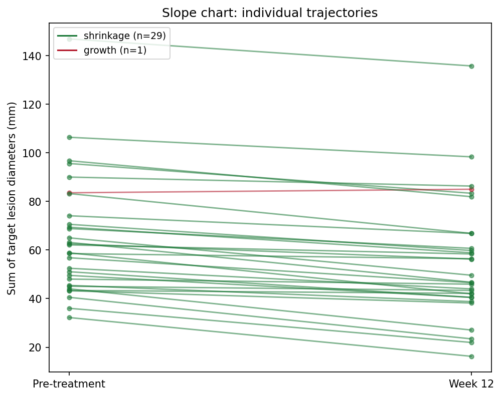
A slope chart with response-direction coloring;
An arrow plot annotated with the paired t-test;
A dumbbell chart sorted by individual change.

Example

Setup

System Requirements: Cross-platform (Linux/MacOS/Windows)
Programming Language: Python
Dependencies: matplotlib, numpy, scipy

import matplotlib.pyplot as plt
import numpy as np
from scipy import stats

Data Preparation

We simulate a Phase-II-style cohort: 30 patients with a sum of target lesion diameters measured at baseline and at week 12. The average effect is a ~9 mm shrinkage, but individual responses vary from strong shrinkage to modest growth — exactly the heterogeneity a paired plot must expose.

rng = np.random.default_rng(5)
n = 30
pre = rng.gamma(shape=4, scale=12, size=n) + 20       # baseline lesion size (mm)
effect = rng.normal(-8, 7, n)                          # individual change
post = np.clip(pre + effect, 8, None)
pid = [f"P{i:02d}" for i in range(1, n + 1)]

delta = post - pre
responders = delta < 0
colors = np.where(responders, "#1B7837", "#B2182B")
t_res = stats.ttest_rel(pre, post)                     # paired t-test
delta.mean(), t_res.pvalue

(np.float64(-9.38768218058284), np.float64(2.9139863594970934e-10))

Visualization

1. Slope Chart

fig, ax = plt.subplots(figsize=(6.8, 5.4))
for i in range(n):
    ax.plot([0, 1], [pre[i], post[i]], color=colors[i], alpha=0.6,
            linewidth=1.4, marker="o", markersize=4)
ax.set_xticks([0, 1]); ax.set_xticklabels(["Pre-treatment", "Week 12"])
ax.set_ylabel("Sum of target lesion diameters (mm)")
handles = [plt.Line2D([], [], color="#1B7837",
                      label=f"shrinkage (n={responders.sum()})"),
           plt.Line2D([], [], color="#B2182B",
                      label=f"growth (n={(~responders).sum()})")]
ax.legend(handles=handles, fontsize=9, loc="upper left")
ax.set_title("Slope chart: individual trajectories")
fig.tight_layout()
plt.show()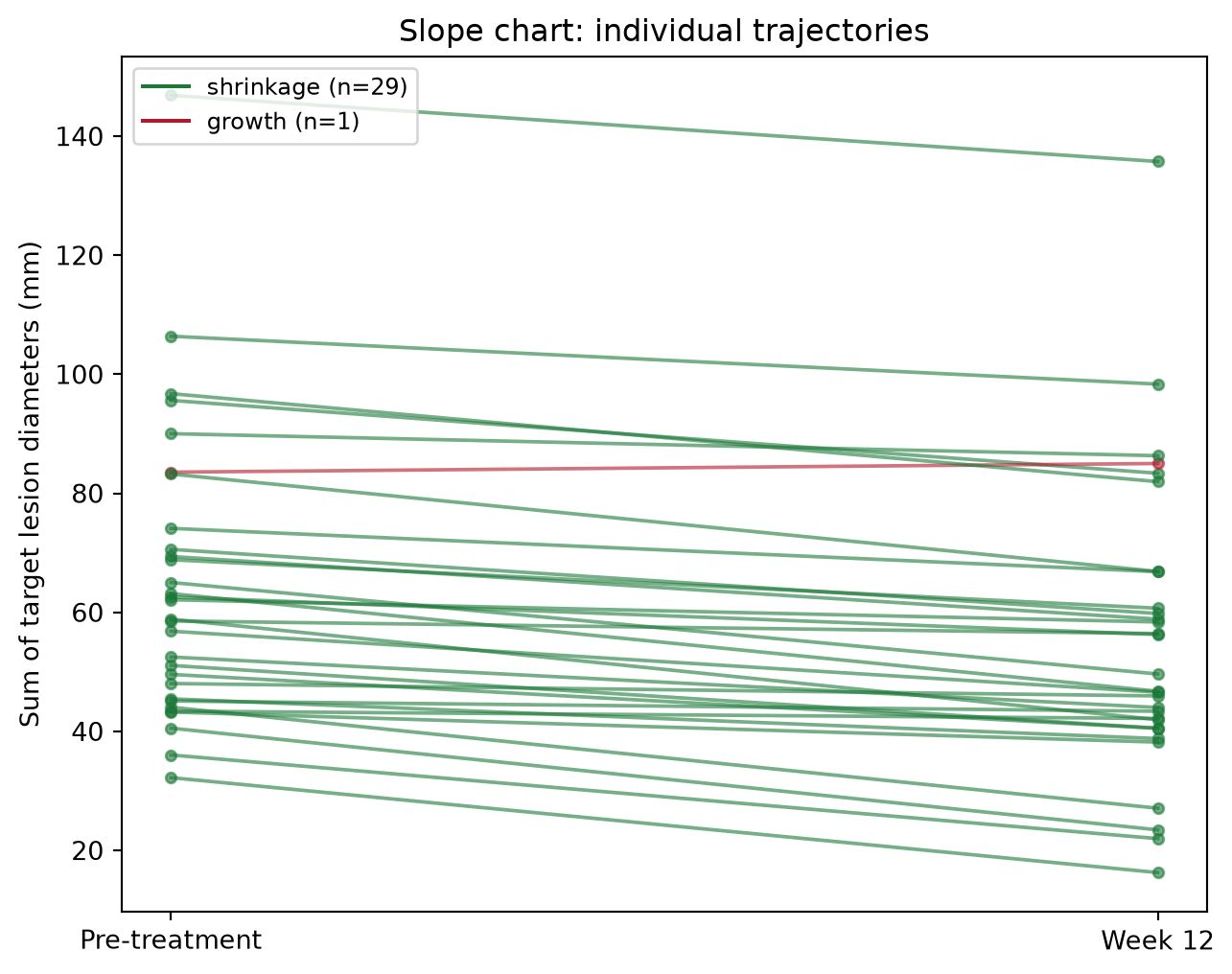

2. Arrow Plot with the Paired t-Test

fig, ax = plt.subplots(figsize=(6.8, 5.4))
ax.scatter(np.zeros(n), pre, s=26, color="#4C72B0", zorder=3, label="pre")
ax.scatter(np.ones(n), post, s=26, color="#B2182B", zorder=3, label="post")
for i in range(n):
    ax.annotate("", xy=(1, post[i]), xytext=(0, pre[i]),
                arrowprops=dict(arrowstyle="->", color=colors[i],
                                alpha=0.65, lw=1.3))
ax.set_xlim(-0.35, 1.35)
ax.set_xticks([0, 1]); ax.set_xticklabels(["Pre", "Week 12"])
ax.set_ylabel("Sum of target lesion diameters (mm)")
ax.text(0.5, ax.get_ylim()[1] * 0.97,
        f"paired t = {t_res.statistic:.2f}, p = {t_res.pvalue:.1e}",
        ha="center", va="top", fontsize=10,
        bbox=dict(boxstyle="round,pad=0.3", fc="#FFF3E0", ec="#E65100"))
ax.legend(loc="lower left", fontsize=9)
ax.set_title("Arrow plot with paired t-test")
fig.tight_layout()
plt.show()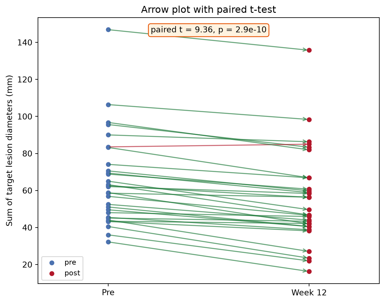

3. Dumbbell Chart Sorted by Change

order = np.argsort(delta)
fig, ax = plt.subplots(figsize=(6.8, 6.2))
y = np.arange(n)
for i, idx in enumerate(order):
    ax.plot([pre[idx], post[idx]], [y[i], y[i]], color=colors[idx],
            alpha=0.6, lw=2)
ax.scatter(pre[order], y, s=30, color="#4C72B0", zorder=3, label="pre")
ax.scatter(post[order], y, s=30, color="#B2182B", zorder=3, label="post")
ax.set_yticks(y); ax.set_yticklabels([pid[i] for i in order], fontsize=7)
ax.set_xlabel("Sum of target lesion diameters (mm)")
ax.axvline(pre.mean(), color="grey", ls=":", lw=1)
ax.legend(loc="lower right", fontsize=9)
ax.set_title("Dumbbell chart sorted by change")
fig.tight_layout()
plt.show()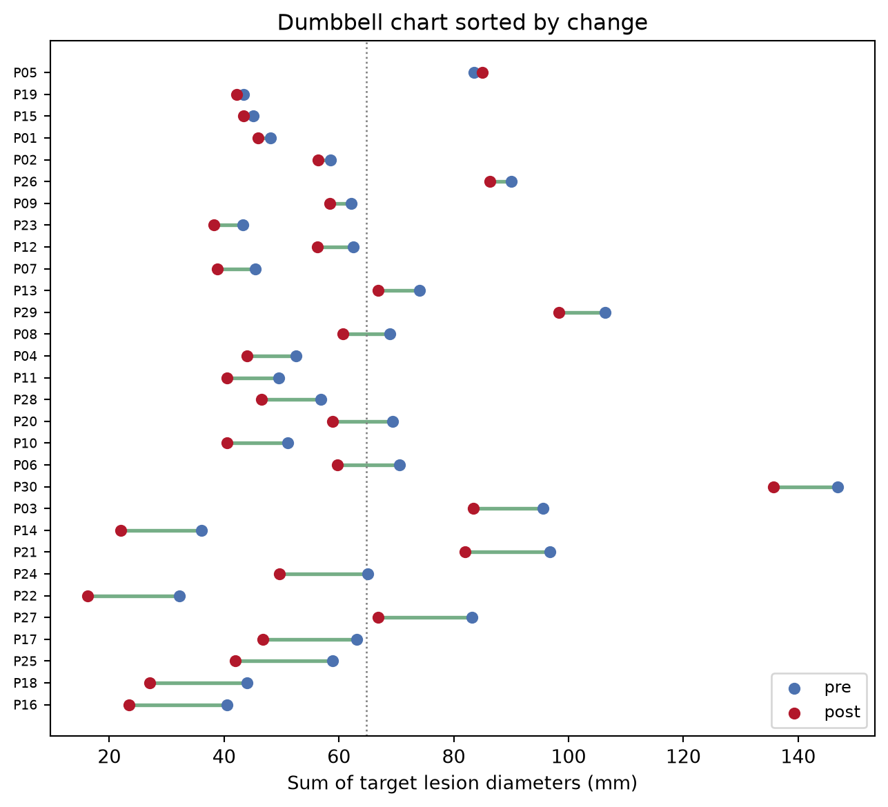

Figure 3: Dumbbell chart sorted by individual change: each patient reads as a bar from pre (blue) to post (red); the sort turns 30 arrows into an effect-size ranking.

Practice tips

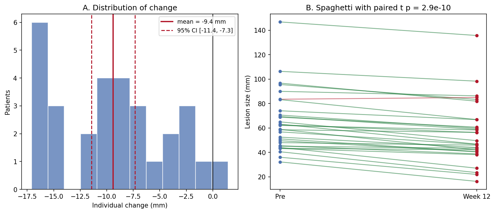
Use scipy.stats.ttest_rel — ttest_ind on paired data throws away the correlation between visits and usually overstates the p-value.
The paired t-test assumes approximately normal differences; check the change histogram (Application panel A) and switch to wilcoxon when it is skewed.
Never summarize a paired design with two unrelated boxplots — the pairing is the design.
Color by response direction, not by visit, so growth cases cannot disappear visually.

Application

The publication-style panel pairs the summary (A: distribution of individual change with mean and 95% CI) with the raw trajectories (B). The CI answers “is there an effect”; the spaghetti answers “is the effect consistent” — reviewers ask both.

Reference

[1] Virtanen P, Gommers R, Oliphant TE, et al. SciPy 1.0: fundamental algorithms for scientific computing in Python. Nat Methods. 2020;17:261-272. doi:10.1038/s41592-019-0686-2