# Install packages
if (!requireNamespace("treemap", quietly = TRUE)) {
  install.packages("treemap")
}
if (!requireNamespace("tidyverse", quietly = TRUE)) {
  install.packages("tidyverse")
}
if (!requireNamespace("stats", quietly = TRUE)) {
  install.packages("stats")
}
if (!requireNamespace("DOSE", quietly = TRUE)) {
  install.packages("DOSE")
}

# Load packages
library(treemap)
library(tidyverse)
library(stats)
library(DOSE)
library(palmerpenguins)Treemap
A treemap, also known as a rectangular tree structure diagram, is composed of multiple nested rectangles of varying areas. The sum of the areas of all rectangles represents the overall data. The area of each smaller rectangle represents the proportion of each sub-item; the larger the rectangle’s area, the larger the proportion of that sub-item within the whole.
Example
Treemap are suitable for displaying data with hierarchical relationships and can intuitively show the comparison between peers (tree diagrams use rectangles of different colors and sizes to display the hierarchical structure of the data).
Setup
System Requirements: Cross-platform (Linux/MacOS/Windows)
Programming Language: R
Dependencies:
treemap;tidyverse;stats;DOSE
sessioninfo::session_info("attached")─ Session info ───────────────────────────────────────────────────────────────
setting value
version R version 4.6.0 (2026-04-24)
os Ubuntu 24.04.4 LTS
system x86_64, linux-gnu
ui X11
language (EN)
collate C.UTF-8
ctype C.UTF-8
tz UTC
date 2026-05-09
pandoc 3.1.3 @ /usr/bin/ (via rmarkdown)
quarto 1.9.37 @ /usr/local/bin/quarto
─ Packages ───────────────────────────────────────────────────────────────────
package * version date (UTC) lib source
DOSE * 4.6.0 2026-04-28 [1] Bioconduc~
dplyr * 1.2.1 2026-04-03 [1] RSPM
forcats * 1.0.1 2025-09-25 [1] RSPM
ggplot2 * 4.0.3.9000 2026-05-04 [1] Github (tidyverse/ggplot2@6870419)
lubridate * 1.9.5 2026-02-04 [1] RSPM
palmerpenguins * 0.1.1 2022-08-15 [1] RSPM
purrr * 1.2.2 2026-04-10 [1] RSPM
readr * 2.2.0 2026-02-19 [1] RSPM
stringr * 1.6.0 2025-11-04 [1] RSPM
tibble * 3.3.1 2026-01-11 [1] RSPM
tidyr * 1.3.2 2025-12-19 [1] RSPM
tidyverse * 2.0.0 2023-02-22 [1] RSPM
treemap * 2.4-4 2023-05-25 [1] RSPM
[1] /home/runner/work/_temp/Library
[2] /opt/R/4.6.0/lib/R/site-library
[3] /opt/R/4.6.0/lib/R/library
* ── Packages attached to the search path.
──────────────────────────────────────────────────────────────────────────────Data Preparation
data_USArrests <- rownames_to_column(USArrests[1:8,], "State")

data_swiss <- swiss

data_countsub <- aggregate(penguins, by=list(penguins$species, penguins$sex),length)
data_countsub <- data_countsub[ ,1:3]
colnames(data_countsub) <- c("species", "sex", "count")

data_BP <- readr::read_csv("https://bizard-1301043367.cos.ap-guangzhou.myqcloud.com/data_BP.csv")
data_BP <- data_BP[order(abs(data_BP$NES), decreasing = T),]
data_BP <- data_BP[1:13,]

data_KEGG_type <- readr::read_csv("https://bizard-1301043367.cos.ap-guangzhou.myqcloud.com/data_KEGG.csv")
data_KEGG_type$pvalue_log <- -log10(data_KEGG_type$pvalue)
Visualization
1. Single variable classification
1.1 Color according to the label
Taking the USArrests dataset as an example
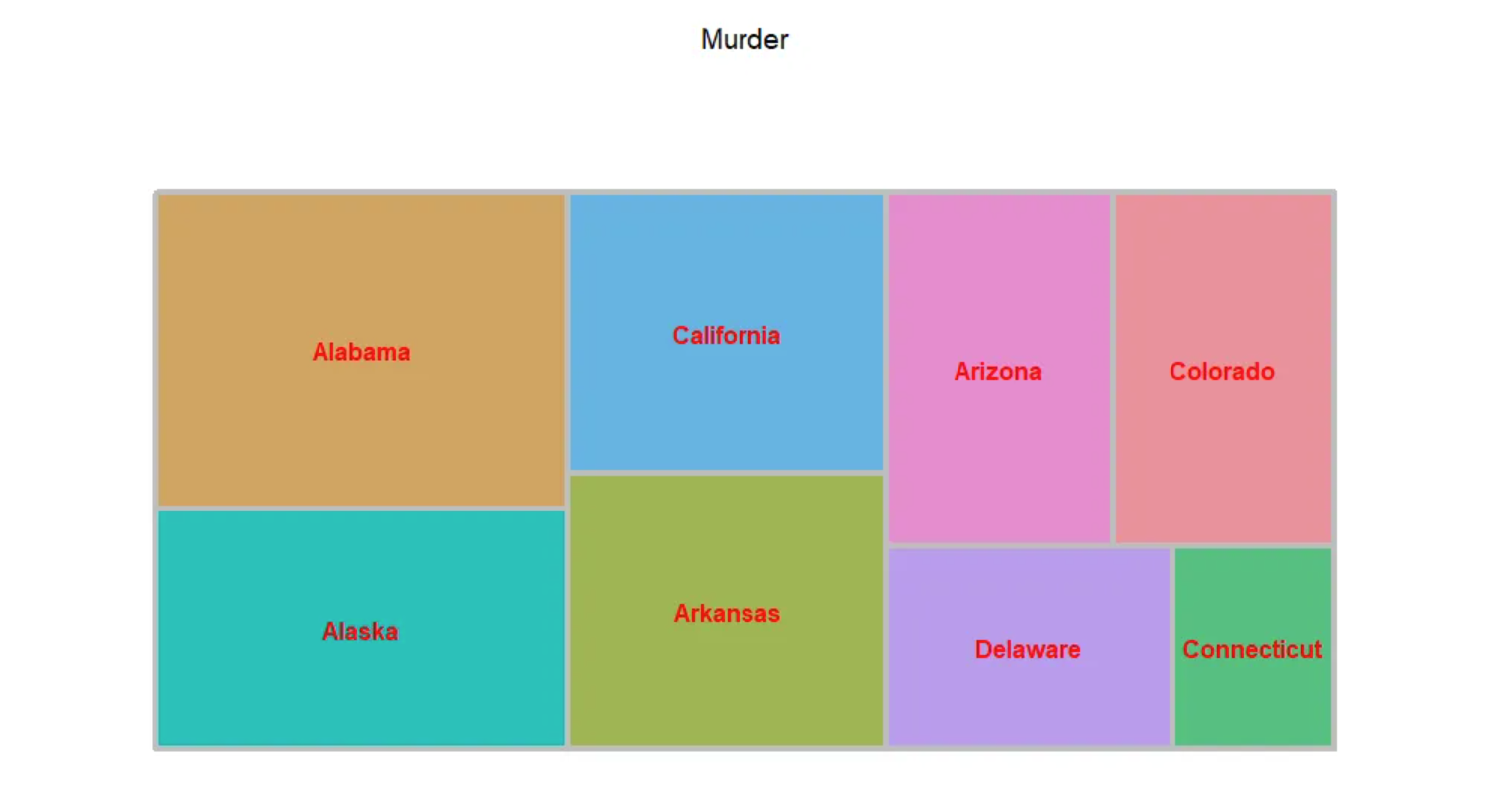
treemap(data_USArrests, # data
        index = "State", # Categorical variables
        vSize = "Murder", # Categorical variable corresponding data values
        vColor="State", # The corresponding columns of color depth, here the data size is used as the corresponding
        type = "index", # Color mapping method, including "index", "value", "comp", "dens", "depth", "categorical", "color", and "manual".
        title = 'Murder', # title
        border.col = "grey", # Border color
        border.lwds = 4, # Border line width
        fontsize.labels = 12, # Label size
        fontcolor.labels = 'red', # Label color
        align.labels = list(c("center", "center")), # Tag location
        fontface.labels = 2) # Tag fonts: 1, 2, 3, 4 represent normal, bold, italic, and bold italic fonts, respectively.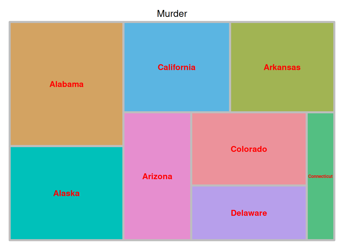
The image above is a tree diagram showing the proportion of criminal arrests in different U.S. states, with each state used as the basis for coloring.
1.2 Color according to data size
Taking the USArrests dataset as an example
treemap(data_USArrests,
        index = "State",
        vSize = "Murder",
        vColor="Murder",
        type = "value",
        title = 'Murder',
        border.col = "grey",
        border.lwds = 4,
        fontsize.labels = 12,
        fontcolor.labels = 'red',
        align.labels = list(c("center", "center")),
        fontface.labels = 2)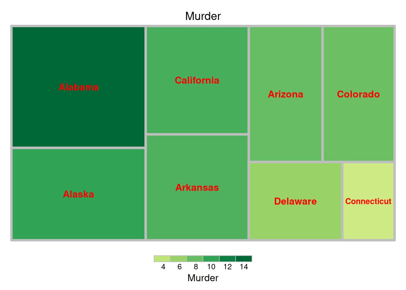
The image above is a tree diagram showing the proportion of criminal arrests in different US states, with color coding based on the size of each data group.
Example: Hallmark analysis data of differentially expressed genes in mouse lung tissue before and after cisplatin administration.
treemap(data_BP[1:13,],
        index = "BP",
        vSize = "pvalue_log",
        vColor="NES",
        type = "value",
        title = 'Biological Process',
        border.col = "grey",
        border.lwds = 4,
        fontsize.labels = 10,
        fontcolor.labels = 'white',
        align.labels = list(c("center", "center")),
        fontface.labels = 2)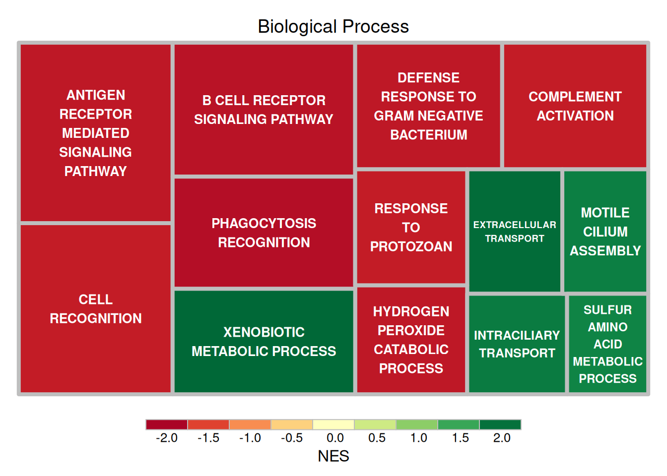
The figure above shows the results of Hallmark analysis of differentially expressed genes in mouse lung tissue before and after cisplatin administration. The size of the rectangle represents the negative value of log10(P), and the larger the rectangle, the more reliable the result. The color of the rectangle represents the NES value.
2. Multivariate classification
Multi-level grouping can be achieved using index = c("Group1", "Group2", ...).
2.1 Color matching based on data labels
Taking the penguins dataset as an example
treemap(data_countsub,
        index = c("sex","species"),
        vSize = "count",
        vColor="species",
        type = "index",
        title = 'Count',
        border.col = c("black","white"),
        border.lwds = c(4,1),
        fontsize.labels = c(18,10),
        bg.labels=c("transparent"),
        fontcolor.labels = c('white',"orange"),
        align.labels = list(c("left", "top"),
                            c("center", "center")),
        fontface.labels = c(2,3))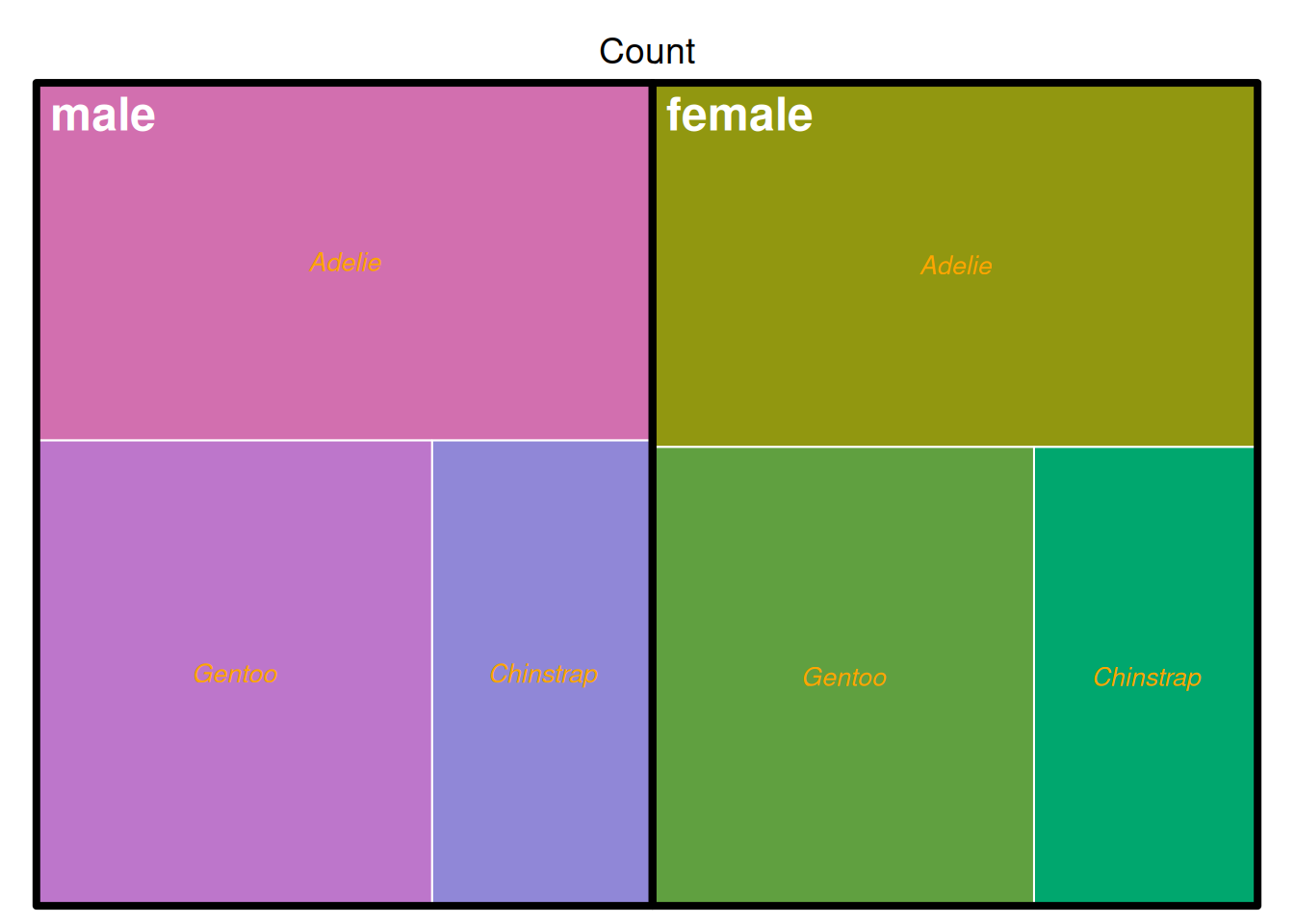
The image above shows the penguin counts in the penguins dataset, grouped by sex and species. The classification is used as the basis for coloring.
2.2 Color according to data size
Taking the penguins dataset as an example
treemap(data_countsub,
        index = c("sex","species"),
        vSize = "count",
        vColor="count",
        type = "value",
        title = 'Count',
        border.col = c("black","white"),
        border.lwds = c(4,1),
        fontsize.labels = c(18,10),
        bg.labels=c("transparent"),
        fontcolor.labels = c('white',"orange"),
        align.labels = list(c("left", "top"),
                            c("center", "center")),
        fontface.labels = c(2,3))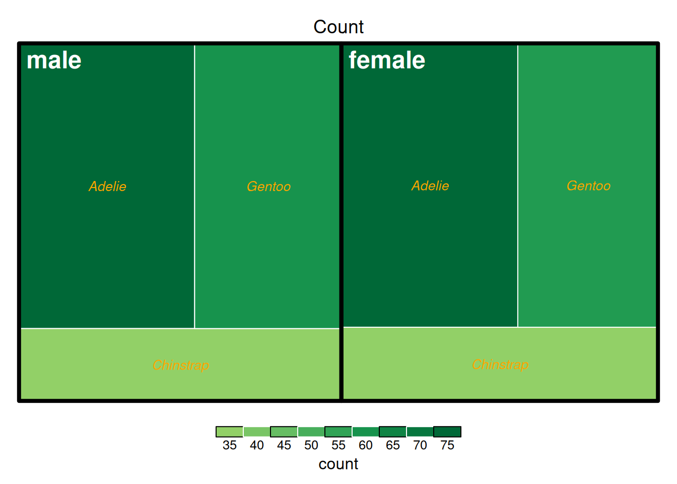
The image above shows the penguin counts in the penguins dataset, grouped by sex and species. The coloring is based on the count.
The following example uses pathway analysis data of differentially expressed genes in mouse lung tissue before and after cisplatin administration.
treemap(data_KEGG_type,
        index = c("type","subtype","PW"),
        vSize = "pvalue_log",
        vColor="NES",
        type = "value",
        title = 'KEGG pathway analysis results data',
        border.col = c("black","white","orange"),
        border.lwds = c(4,1),
        fontsize.labels = c(18,15,10),
        bg.labels=c("transparent"),
        fontcolor.labels = c('black',"white","orange"),
        align.labels = list(c("left", "top"),
                            c("center", "center"),
                            c("left","bottom")),
        fontface.labels = c(2,3))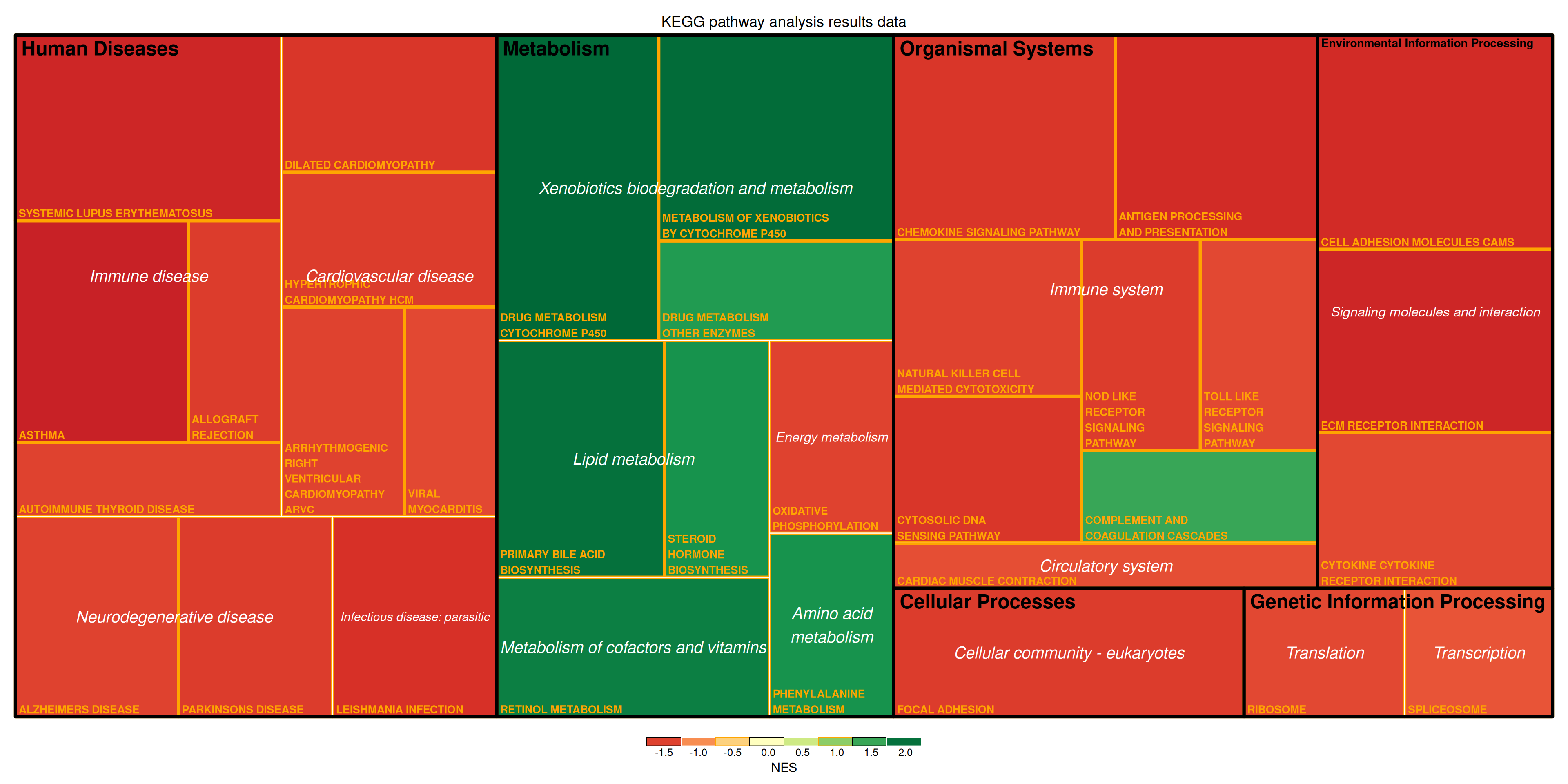
The figure above shows the KEGG pathway analysis results for differentially expressed genes in mouse lung tissue before and after cisplatin treatment. The figure illustrates the multi-level classification of pathways. The size of the rectangle represents the negative log10(P) value, with larger rectangles indicating more reliable results. The color of the rectangles represents the Negative Estimates (NES) value.
Applications
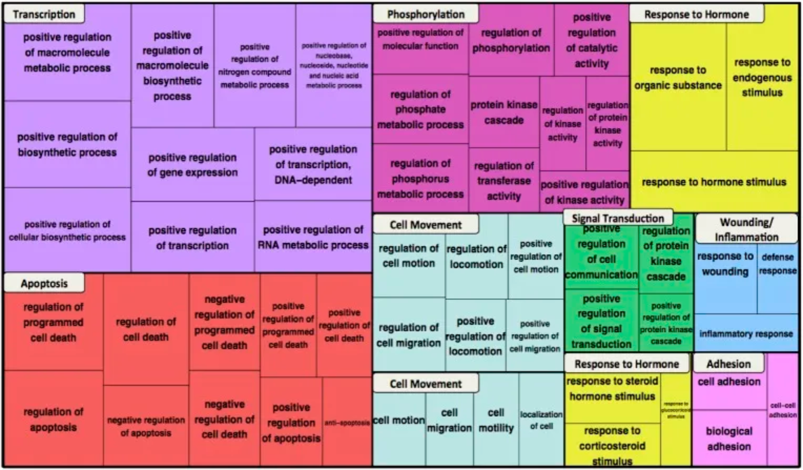
The figure above shows the functional enrichment of GO biological process terms for the β-catenin network. The most enriched terms in the top ten clusters are shown in the dendrogram, represented by color blocks. For each term, the box size reflects the p-value for term enrichment. [1]
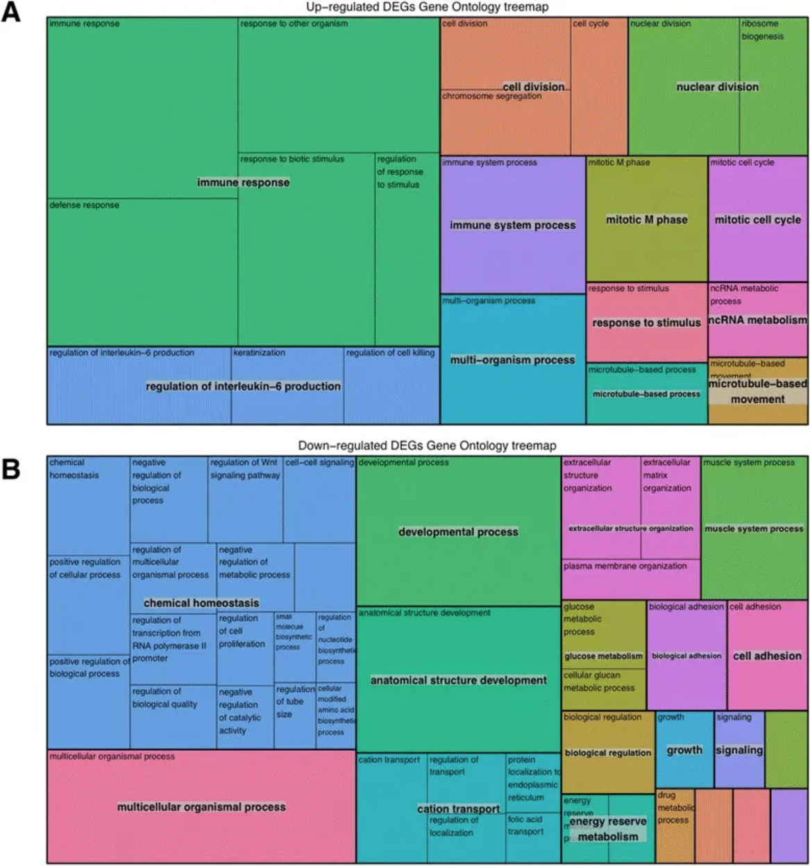
The figure above shows the gene analysis of upregulated and downregulated genes. BiNGO was used to perform gene analysis on upregulated and downregulated genes. Existence arguments and associated correction p-values were passed to REVIGO, which performed a summary by removing redundant GO terms.
A tree diagram with functional annotations associated with (a) upregulated and (b) downregulated genes was generated. [2]
Reference
[1] Çelen İ, Ross KE, Arighi CN, Wu CH. Bioinformatics Knowledge Map for Analysis of Beta-Catenin Function in Cancer. PLoS One. 2015 Oct 28;10(10):e0141773. doi: 10.1371/journal.pone.0141773. PMID: 26509276; PMCID: PMC4624812.
[2] Corley SM, Canales CP, Carmona-Mora P, Mendoza-Reinosa V, Beverdam A, Hardeman EC, Wilkins MR, Palmer SJ. RNA-Seq analysis of Gtf2ird1 knockout epidermal tissue provides potential insights into molecular mechanisms underpinning Williams-Beuren syndrome. BMC Genomics. 2016 Jun 13;17:450. doi: 10.1186/s12864-016-2801-4. PMID: 27295951; PMCID: PMC4907016.
[3] Tennekes M (2023). treemap: Treemap Visualization. R package version 2.4-4, https://CRAN.R-project.org/package=treemap.
[4] Wickham H, Averick M, Bryan J, Chang W, McGowan LD, François R, Grolemund G, Hayes A, Henry L, Hester J, Kuhn M, Pedersen TL, Miller E, Bache SM, Müller K, Ooms J, Robinson D, Seidel DP, Spinu V, Takahashi K, Vaughan D, Wilke C, Woo K, Yutani H (2019). “Welcome to the tidyverse.” Journal of Open Source Software, 4(43), 1686. doi:10.21105/joss.01686 https://doi.org/10.21105/joss.01686.
[5] R Core Team (2024). R: A Language and Environment for Statistical Computing. R Foundation for Statistical Computing, Vienna, Austria. https://www.R-project.org/.