Oceania/Antarc Map

Authors

[Editor] Hu Zheng;

[Contributors]

Modified

2026-01-17

Note

Hiplot website

This page is the tutorial for source code version of the Hiplot Oceania/Antarc Map plugin. You can also use the Hiplot website to achieve no code ploting. For more information please see the following link:

https://hiplot.cn/basic/map-oceania-antarc?lang=en

Setup

System Requirements: Cross-platform (Linux/MacOS/Windows)
Programming language: R
Dependent packages: data.table; jsonlite; ggplot2; RColorBrewer

# Install packages
if (!requireNamespace("data.table", quietly = TRUE)) {
  install.packages("data.table")
}
if (!requireNamespace("jsonlite", quietly = TRUE)) {
  install.packages("jsonlite")
}
if (!requireNamespace("ggplot2", quietly = TRUE)) {
  install.packages("ggplot2")
}
if (!requireNamespace("RColorBrewer", quietly = TRUE)) {
  install.packages("RColorBrewer")
}

# Load packages
library(data.table)
library(jsonlite)
library(ggplot2)
library(RColorBrewer)

sessioninfo::session_info("attached")

─ Session info ───────────────────────────────────────────────────────────────
 setting  value
 version  R version 4.5.2 (2025-10-31)
 os       Ubuntu 24.04.3 LTS
 system   x86_64, linux-gnu
 ui       X11
 language (EN)
 collate  C.UTF-8
 ctype    C.UTF-8
 tz       UTC
 date     2026-01-17
 pandoc   3.1.3 @ /usr/bin/ (via rmarkdown)
 quarto   1.8.27 @ /usr/local/bin/quarto

─ Packages ───────────────────────────────────────────────────────────────────
 package      * version date (UTC) lib source
 data.table   * 1.18.0  2025-12-24 [1] RSPM
 ggplot2      * 4.0.1   2025-11-14 [1] RSPM
 jsonlite     * 2.0.0   2025-03-27 [1] RSPM
 RColorBrewer * 1.1-3   2022-04-03 [1] RSPM

 [1] /home/runner/work/_temp/Library
 [2] /opt/R/4.5.2/lib/R/site-library
 [3] /opt/R/4.5.2/lib/R/library
 * ── Packages attached to the search path.

──────────────────────────────────────────────────────────────────────────────

Data Preparation

# Load data
data <- data.table::fread(jsonlite::read_json("https://hiplot.cn/ui/basic/map-oceania-antarc/data.json")$exampleData$textarea[[1]])
data <- as.data.frame(data)
dt_map <- readRDS(url("https://download.hiplot.cn/ui/basic/map-oceania-antarc/oca.rds"))

# Convert data structure
dt_map$Value <- data$value[match(dt_map$ENG_NAME, data$region)]

# View data
head(data)

                      region value
1        American Samoa (US)   672
2                 Antarctica     3
3    Pacific Is Refuges (US)   320
4 Cook Islands (NEW ZEALAND)   740
5                       FIJI   303
6  French Polynesia (FRANCE)   879

Visualization

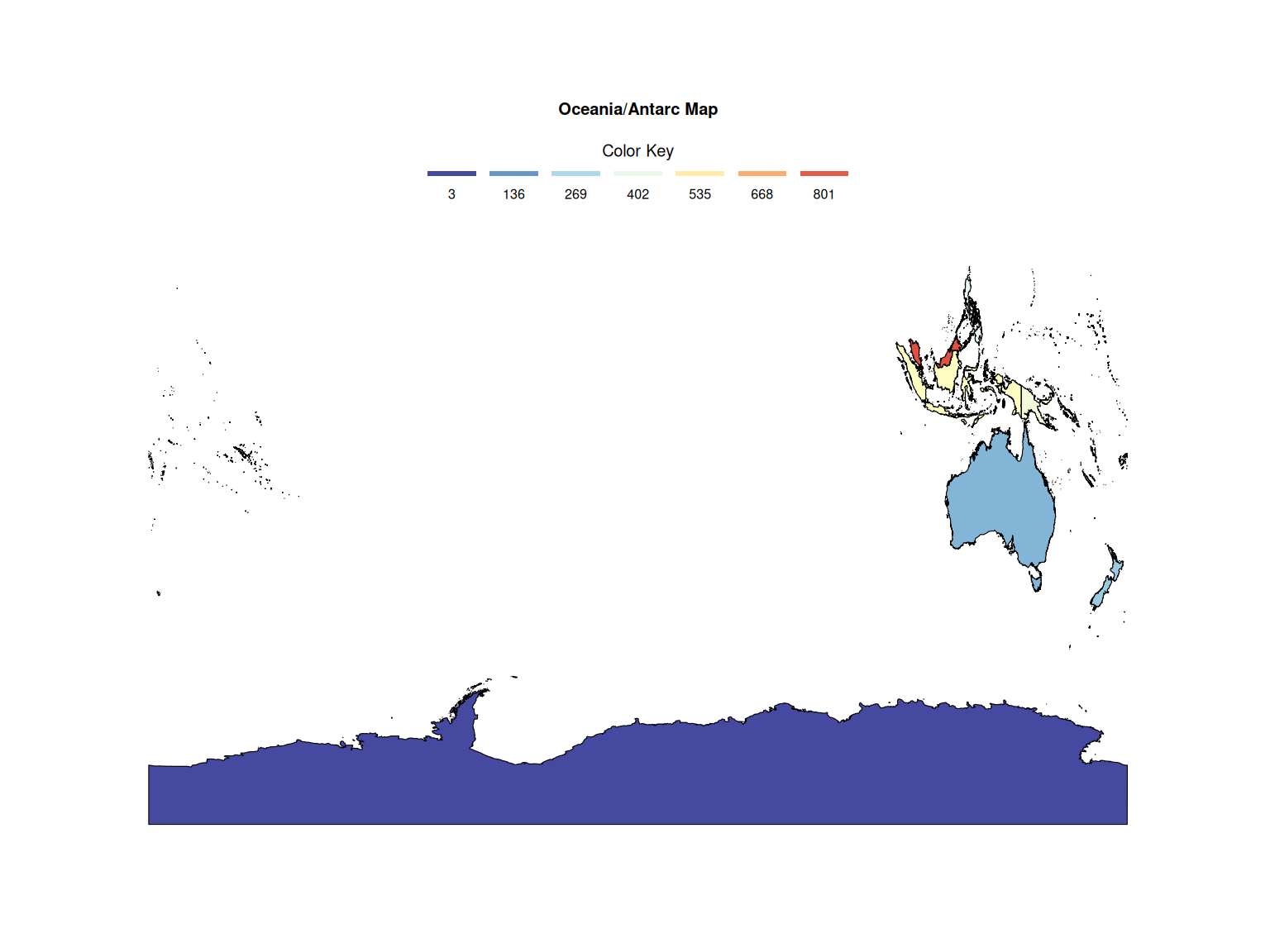
# Oceania/Antarc Map
p <- ggplot(dt_map) +
  geom_polygon(aes(x = long, y = lat, group = group, fill = Value),
               alpha = 0.9, size = 0.5) +
  geom_path(aes(x = long, y = lat, group = group), color = "black", size = 0.2) +
  coord_fixed() +
  scale_fill_gradientn(
    colours = colorRampPalette(rev(brewer.pal(11,"RdYlBu")))(500),
    breaks = seq(min(data$value), max(data$value), 
                 round((max(data$value)-min(data$value))/7)),
    name = "Color Key",
    guide = guide_legend(
      direction = "vertical", keyheight = unit(1, units = "mm"),
      keywidth = unit(8, units = "mm"),
      title.position = "top", title.hjust = 0.5, label.hjust = 0.5,
      nrow = 1, byrow = T, reverse = F, label.position = "bottom")) +
  theme(text = element_text(color = "#3A3F4A"),
        axis.text = element_blank(),
        axis.ticks = element_blank(),
        panel.grid.major = element_blank(),
        panel.grid.minor = element_blank(),
        legend.position = "top",
        legend.text = element_text(size = 4 * 1.5, color = "black"),
        legend.title = element_text(size = 5 * 1.5, color = "black"),
        plot.title = element_text(
          face = "bold", size = 5 * 1.5, hjust = 0.5, 
          margin = margin(t = 4, b = 5), color = "black"),
        plot.background = element_rect(fill = "#FFFFFF", color = "#FFFFFF"),
        panel.background = element_rect(fill = "#FFFFFF", color = NA),
        legend.background = element_rect(fill = "#FFFFFF", color = NA),
        plot.margin = unit(c(1.5, 1.5, 1.5, 1.5), "cm")) +
  labs(x = NULL, y = NULL, title = "Oceania/Antarc Map")

p