# Install packages
if (!requireNamespace("data.table", quietly = TRUE)) {
  install.packages("data.table")
}
if (!requireNamespace("jsonlite", quietly = TRUE)) {
  install.packages("jsonlite")
}
if (!requireNamespace("plot3D", quietly = TRUE)) {
  install.packages("plot3D")
}
if (!requireNamespace("ggplotify", quietly = TRUE)) {
  install.packages("ggplotify")
}

# Load packages
library(data.table)
library(jsonlite)
library(plot3D)
library(ggplotify)3D-Scatter
Note
Hiplot website
This page is the tutorial for source code version of the Hiplot 3D-Scatter plugin. You can also use the Hiplot website to achieve no code ploting. For more information please see the following link:
3D scatter plot is to apply a number of quantitative variables to different coaxes in space and combine different variables into coordinates in space, so as to clearly explain the interaction between the three quantitative variables.
Setup
System Requirements: Cross-platform (Linux/MacOS/Windows)
Programming language: R
Dependent packages:
data.table;jsonlite;plot3D;ggplotify
sessioninfo::session_info("attached")─ Session info ───────────────────────────────────────────────────────────────
setting value
version R version 4.6.0 (2026-04-24)
os Ubuntu 24.04.4 LTS
system x86_64, linux-gnu
ui X11
language (EN)
collate C.UTF-8
ctype C.UTF-8
tz UTC
date 2026-05-09
pandoc 3.1.3 @ /usr/bin/ (via rmarkdown)
quarto 1.9.37 @ /usr/local/bin/quarto
─ Packages ───────────────────────────────────────────────────────────────────
package * version date (UTC) lib source
data.table * 1.18.4 2026-05-06 [1] RSPM
ggplotify * 0.1.3 2025-09-20 [1] RSPM
jsonlite * 2.0.0 2025-03-27 [1] RSPM
plot3D * 1.4.2 2025-07-25 [1] RSPM
[1] /home/runner/work/_temp/Library
[2] /opt/R/4.6.0/lib/R/site-library
[3] /opt/R/4.6.0/lib/R/library
* ── Packages attached to the search path.
──────────────────────────────────────────────────────────────────────────────Data Preparation
The loaded data are three variables and grouping.
# Load data
data <- data.table::fread(jsonlite::read_json("https://hiplot.cn/ui/basic/scatter-3d/data.json")$exampleData[[1]]$textarea[[1]])
data <- as.data.frame(data)

# Convert data structure
col_idx <- which(colnames(data) == "group")
data[, col_idx] <- as.factor(data[, col_idx])
shapes <- 19
shape_idx <- ""

# View data
head(data)
temp pressure dtime group
1 41.11057 0.49351190 1 G1
2 35.23429 0.76636476 2 G1
3 26.58407 0.63885937 3 G1
4 34.76097 -0.08106332 4 G1
5 25.76521 -0.31731579 5 G1
6 20.30115 -1.91132873 6 G1Visualization
# 3D-Scatter
p <- as.ggplot(function() {
  plot3d <- scatter3D(data[, 1], data[, 2], data[, 3],
    pch = shapes, cex = 1,
    phi = 0, theta = 45, ticktype = "detailed",
    bty = "b2", colkey = FALSE, alpha = 1,
    xlab = colnames(data)[1], ylab = colnames(data)[2],
    zlab = colnames(data)[3],
    main = "3D-Scatter Plot",
    colvar = as.numeric(as.factor(data[, 4])),
    col = c("#e04d39","#5bbad6","#1e9f86")
  )

  legend("right", pch=19, legend = levels(data[, col_idx]),
         cex = 1.1, bty = 'n', xjust = 0.5, horiz = F,
         title = colnames(data)[col_idx],
         col = c("#e04d39","#5bbad6","#1e9f86"))
})

p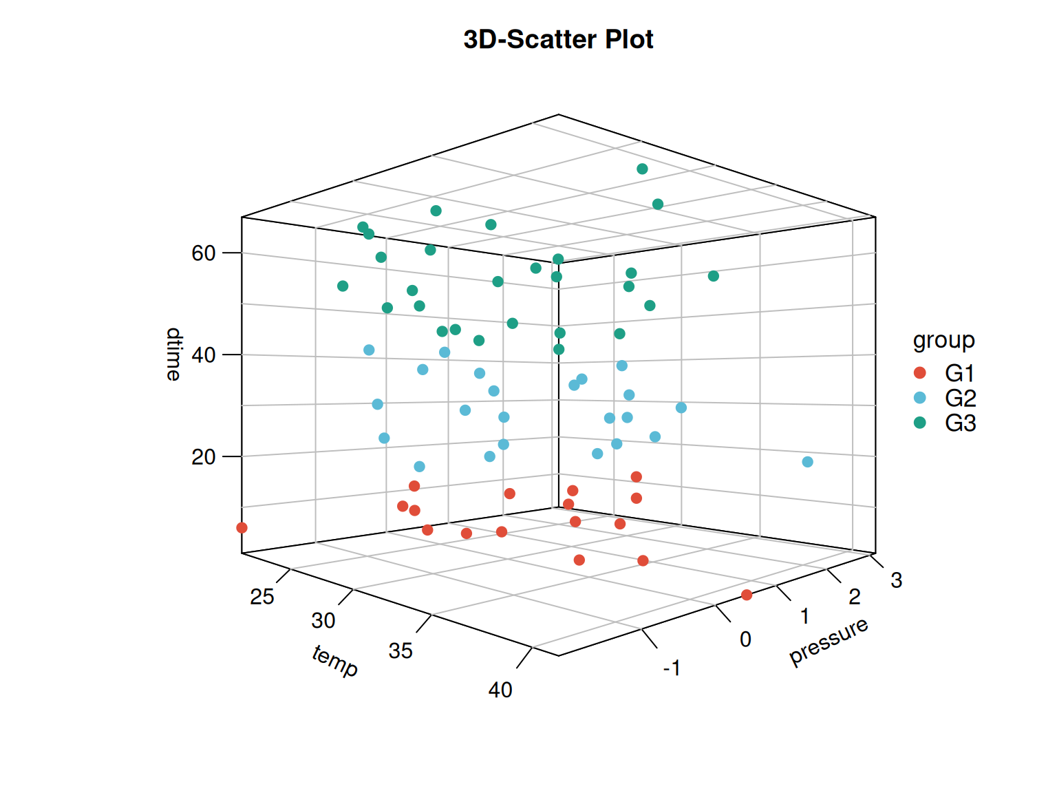
In the figure, temperature, pressure and time are respectively placed on x (horizontal axis), Y (vertical axis) and Z (perspective axis) to generate a THREE-DIMENSIONAL scatter plot, and the correlation between variables and their correlation degree can be intuitively found.