ECDF Plot

Authors

[Contributors] ZCode (GLM) — AI-generated, independently AI-reviewed.

Modified

2026-10-31

🤖 AI Skill — Download the Bizard unified skill for your AI assistant ⬇️ Download Skill ZIP

🔌 MCP Server — Let AI agents (Claude Code, Cursor, …) query Bizard live: claude mcp add bizard -- npx @openbiox/bizard-mcp — or the free hosted instance (no install, faster from mainland China): claude mcp add --transport http bizard http://biotree.top:38123/bizard-mcp/mcp 📖 MCP Docs

📖 Cite Bizard — if Bizard helps your research, please cite: Li, K., Zheng, H., Huang, K., et al. (2026). Bizard: A Community-Driven Platform for Accelerating and Enhancing Biomedical Data Visualization. iMetaMed, e70038. 🔗 DOI / BibTeX

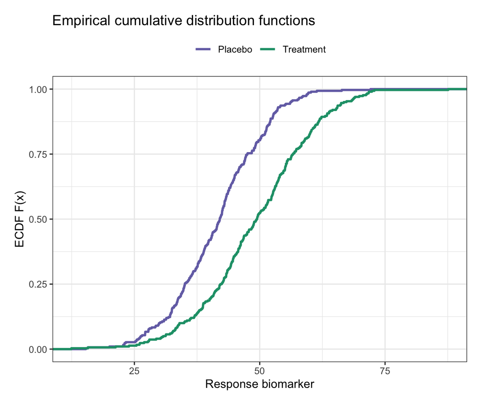
The empirical cumulative distribution function (ECDF), \(F_n(x) = \frac{1}{n}\sum_i \mathbf{1}(x_i \le x)\), plots every observation as a step that climbs from 0 to 1 — a complete, assumption-free portrait of a distribution. Compared with histograms it needs no bin-width tuning, shows every data point’s position, and makes quantiles directly readable: the group median is simply where its curve crosses 0.5 [1]. Two ECDF curves on one axes are also the geometric basis of the two-sample Kolmogorov–Smirnov test — the vertical gap between them is the KS statistic [2].

This tutorial covers four workflows:

Two-group ECDFs with stat_ecdf();
Multi-group ECDFs with annotated medians;
The two-sample ECDF difference plot — visualizing the KS statistic;
The p-value ECDF, a standard omics quality-control view.

Example

Setup

System Requirements: Cross-platform (Linux/MacOS/Windows)
Programming language: R
Dependent packages: ggplot2; dplyr

# Load packages
library(ggplot2)
library(dplyr)

sessioninfo::session_info("attached")

─ Session info ───────────────────────────────────────────────────────────────
 setting  value
 version  R version 4.6.2 (2026-10-29)
 os       Ubuntu 24.04.5 LTS
 system   x86_64, linux-gnu
 ui       X11
 language (EN)
 collate  C.UTF-8
 ctype    C.UTF-8
 tz       UTC
 date     2026-10-31
 pandoc   3.1.3 @ /usr/bin/ (via rmarkdown)
 quarto   1.10.20 @ /usr/local/bin/quarto

─ Packages ───────────────────────────────────────────────────────────────────
 ! package * version    date (UTC) lib source
 P dplyr   * 1.2.1      2026-04-03 [?] RSPM
 P ggplot2 * 4.0.3.9000 2026-10-30 [?] Github (tidyverse/ggplot2@b638d65)

 [1] /home/runner/.cache/R/renv/library/Bizard-5140bdc6/linux-ubuntu-noble/R-4.6/x86_64-pc-linux-gnu
 [2] /home/runner/work/_temp/Library
 [3] /opt/R/4.6.2/lib/R/library

 * ── Packages attached to the search path.
 P ── Loaded and on-disk path mismatch.

──────────────────────────────────────────────────────────────────────────────

Data Preparation

Two seeded datasets: a two-arm biomarker study (Placebo vs Treatment, n = 300 each) and a three-gene expression comparison; plus 2,000 simulated p-values under the null and under a mixture with true signals, for the QC view.

set.seed(251)

resp <- data.frame(
  value = c(rnorm(300, 42, 9), rnorm(300, 49, 11)),
  group = rep(c("Placebo", "Treatment"), each = 300))

set.seed(42)
expr3 <- data.frame(
  expr = c(rnorm(200, 6, 1.4), rnorm(200, 5.4, 1.6), rnorm(200, 4.6, 1.2)),
  gene = rep(c("HER2", "EGFR", "KRAS"), each = 200))

pv_null <- runif(2000)
pv_mix  <- c(runif(1800), 10^(-rnorm(200, 2.4, 0.5)))
pvdf <- data.frame(p = c(pv_null, pv_mix),
                   what = rep(c("Null p-values", "With true signals"), each = 2000))

Visualization

1. Two-Group ECDFs

ggplot(resp, aes(value, colour = group)) +
  stat_ecdf(geom = "step", linewidth = 1) +
  scale_color_manual(values = c(Placebo = "#7570B3", Treatment = "#1B9E77"),
                     name = NULL) +
  labs(x = "Response biomarker", y = "ECDF F(x)",
       title = "Empirical cumulative distribution functions") +
  theme_bw(base_size = 11) +
  theme(legend.position = "top")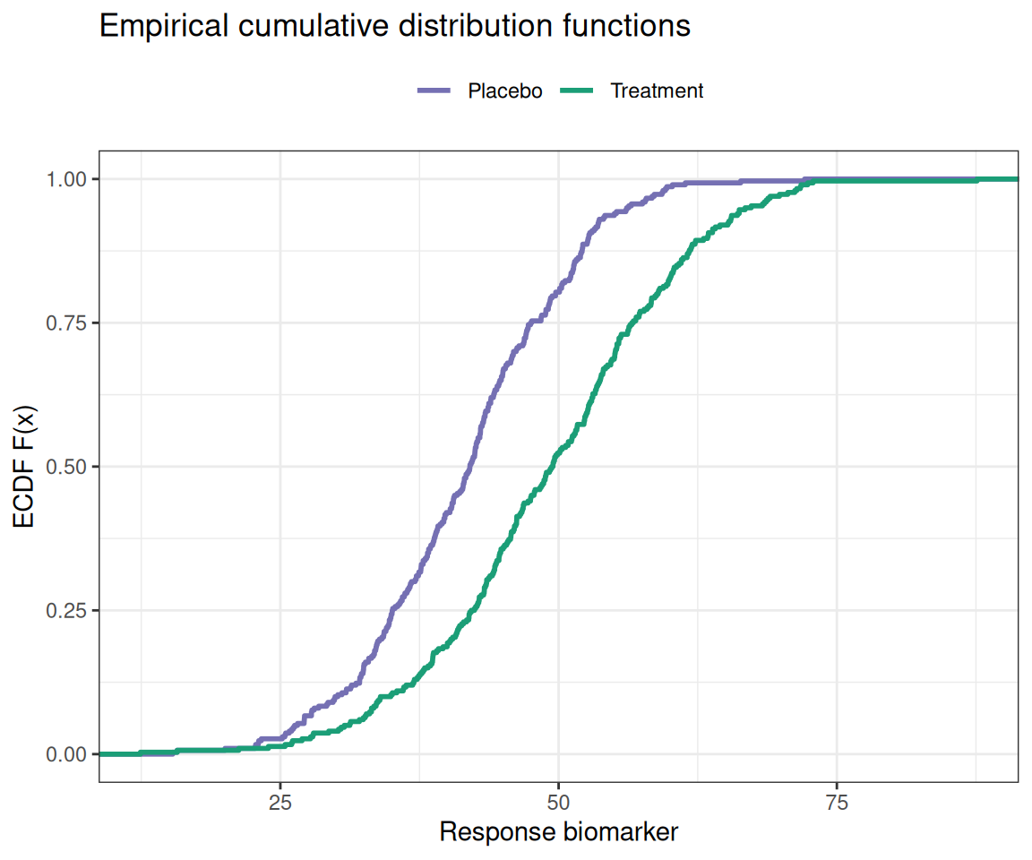

Figure 1: ECDFs of the two arms: the Treatment curve lies to the right of Placebo at every quantile — higher values throughout the distribution, not only on average.

A left-shifted curve means smaller values everywhere: the whole distribution moves, which a difference in means alone cannot establish.

2. Multi-Group ECDFs with Medians

med <- expr3 |>
  group_by(gene) |>
  summarise(med = median(expr))

ggplot(expr3, aes(expr, colour = gene)) +
  stat_ecdf(geom = "step", linewidth = 0.9) +
  geom_point(data = med, aes(med, 0.5), shape = 8, size = 2.6,
             inherit.aes = FALSE, colour = "black") +
  scale_color_brewer(palette = "Dark2", name = NULL) +
  labs(x = "Expression (log2 TPM)", y = "ECDF",
       title = "Stars mark group medians (F(x) = 0.5)") +
  theme_bw(base_size = 11) +
  theme(legend.position = "top")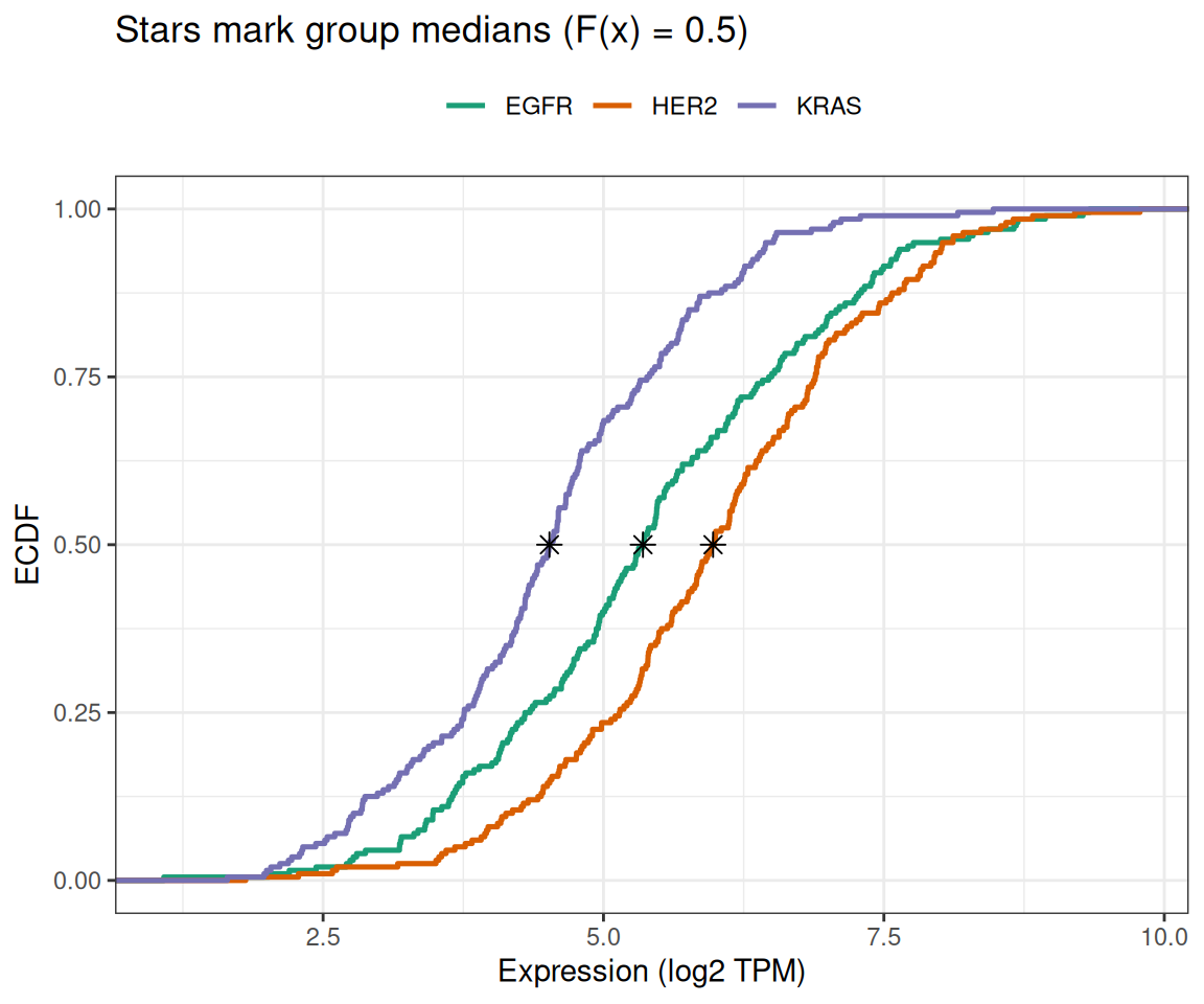

Figure 2: Three-gene expression ECDFs; stars mark each group’s median (where F(x) = 0.5).

3. The ECDF Difference Plot (KS Statistic)

ks <- ks.test(resp$value[resp$group == "Treatment"],
              resp$value[resp$group == "Placebo"])
e1 <- ecdf(resp$value[resp$group == "Treatment"])
e2 <- ecdf(resp$value[resp$group == "Placebo"])
grid <- seq(min(resp$value), max(resp$value), length.out = 600)
dd <- data.frame(x = grid, d = e1(grid) - e2(grid))
imax <- which.max(abs(dd$d))

ggplot(dd, aes(x, d)) +
  geom_line(color = "#1B7837", linewidth = 1) +
  geom_hline(yintercept = 0, linetype = "dashed", color = "grey45") +
  geom_point(data = dd[imax, ], aes(x, d), color = "#B2182B", size = 2.6) +
  annotate("text", x = dd$x[imax], y = max(abs(dd$d)), vjust = -0.8,
           size = 3.4, color = "#B2182B",
           label = sprintf("D = %.2f, KS p = %.2g", max(abs(dd$d)), ks$p.value)) +
  labs(x = "Response biomarker", y = "ECDF(Treatment) - ECDF(Placebo)",
       title = "Two-sample ECDF difference (Kolmogorov-Smirnov)") +
  theme_bw(base_size = 11)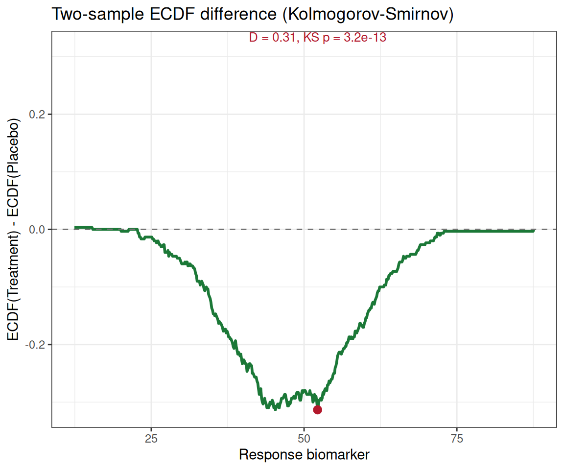

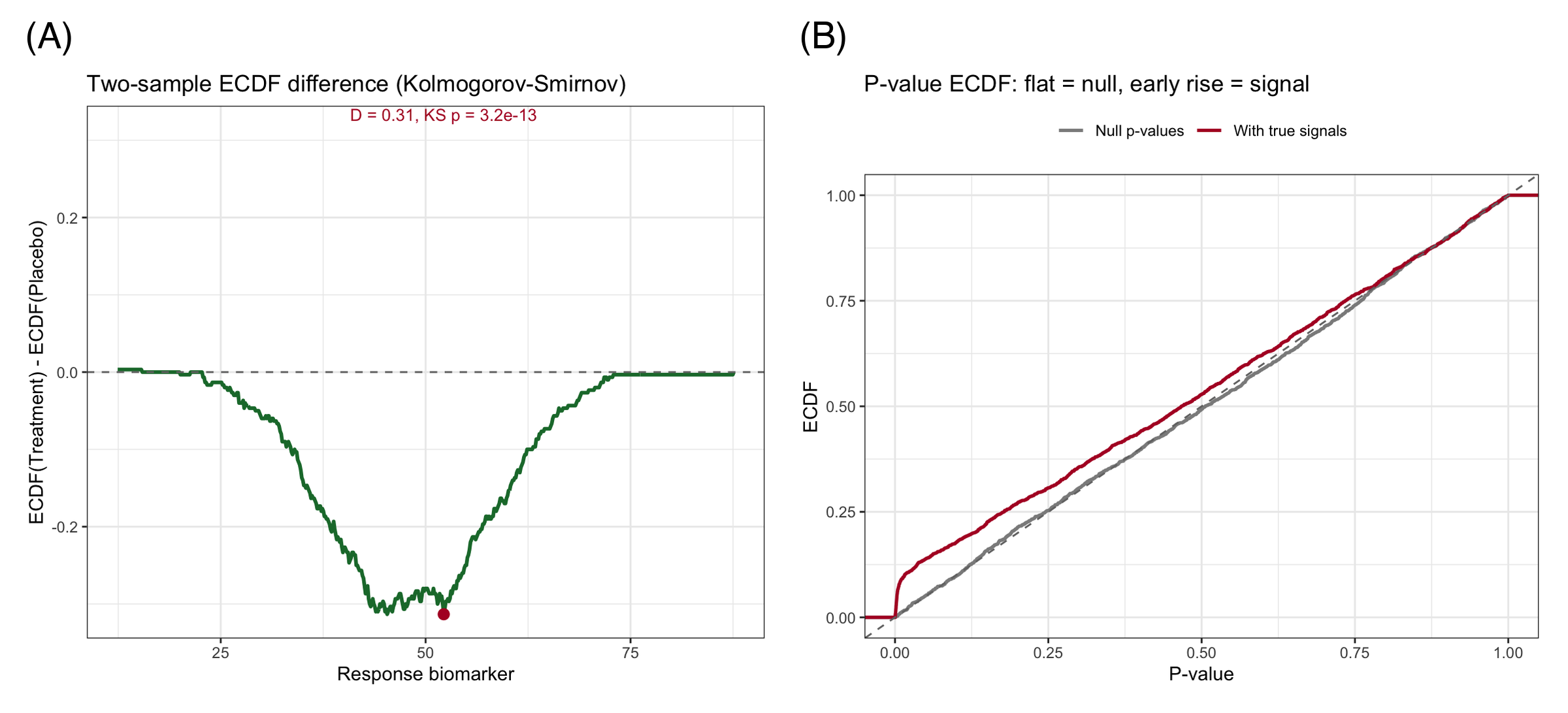
Figure 3: ECDF(Treatment) minus ECDF(Placebo): the largest absolute vertical gap is the Kolmogorov-Smirnov statistic (D = 0.31, p = 3.2e-13).

This figure shows where the distributions differ, not just that they differ — here the gap peaks near the middle of the range and shrinks in the tails.

4. The P-Value ECDF (Omics QC View)

Under a true null, p-values are Uniform(0,1) and their ECDF hugs the diagonal. True signals push small p-values into the population, and the ECDF rises early — making this a one-glance calibration check for any large-scale testing pipeline.

ggplot(pvdf, aes(p, colour = what)) +
  stat_ecdf(geom = "step", linewidth = 0.9) +
  geom_abline(intercept = 0, slope = 1, linetype = "dashed", color = "grey45") +
  scale_color_manual(values = c("Null p-values" = "grey55",
                                "With true signals" = "#B2182B"), name = NULL) +
  labs(x = "P-value", y = "ECDF",
       title = "P-value ECDF: flat = null, early rise = signal") +
  theme_bw(base_size = 11) +
  theme(legend.position = "top")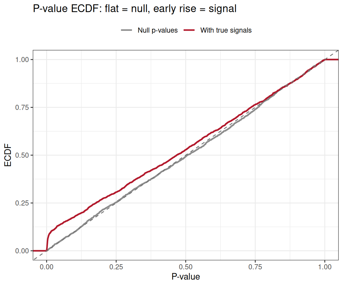

Figure 4: ECDF of p-values: null p-values track the diagonal, while the mixture with true signals rises early (enrichment of small p-values).

Practice tips

ECDFs reveal sample size: the number of steps is n — do not publish them if revealing n is a problem.
Read quantiles off the y-axis: F(x) = 0.25 / 0.5 / 0.75 crossings are the quartiles — annotate them when the audience is clinical.
For right-skewed data, plot the ECDF on a log x-axis (scale_x_log10()) — the monotone shape survives the transform, the readability does not.
Heavy-tailed “complementary” view: plot 1 − F(x) on a log y scale to expose upper-tail behavior (survival-style).

Application

ECDF plots serve distribution comparison wherever medians and tails matter more than means: drug-response screening (per-plate EC50 shifts), flow cytometry marker shifts, differential-expression p-value QC, and wait-time/service data in health-services research. The panel below mirrors a typical publication layout: (A) two-group ECDFs with medians and (B) the KS difference plot.

Reference

[1] Chambers JM, Cleveland WS, Kleiner B, Tukey PA. Graphical Methods for Data Analysis. Belmont: Wadsworth; 1983.

[2] Hodges JL. The significance probability of the Smirnov two-sample test. Ark Mat. 1957;3(5):469-486. doi:10.1007/BF02589501