# Install packages
if (!requireNamespace("data.table", quietly = TRUE)) {
  install.packages("data.table")
}
if (!requireNamespace("jsonlite", quietly = TRUE)) {
  install.packages("jsonlite")
}
if (!requireNamespace("ggplot2", quietly = TRUE)) {
  install.packages("ggplot2")
}
if (!requireNamespace("dplyr", quietly = TRUE)) {
  install.packages("dplyr")
}
if (!requireNamespace("ggrepel", quietly = TRUE)) {
  install.packages("ggrepel")
}

# Load packages
library(data.table)
library(jsonlite)
library(ggplot2)
library(dplyr)
library(ggrepel)Connected Scatterplot
Note
Hiplot website
This page is the tutorial for source code version of the Hiplot Connected Scatterplot plugin. You can also use the Hiplot website to achieve no code ploting. For more information please see the following link:
Connected scatterplot
Setup
System Requirements: Cross-platform (Linux/MacOS/Windows)
Programming language: R
Dependent packages:
data.table;jsonlite;ggplot2;dplyr;ggrepel
sessioninfo::session_info("attached")─ Session info ───────────────────────────────────────────────────────────────
setting value
version R version 4.6.0 (2026-04-24)
os Ubuntu 24.04.4 LTS
system x86_64, linux-gnu
ui X11
language (EN)
collate C.UTF-8
ctype C.UTF-8
tz UTC
date 2026-05-09
pandoc 3.1.3 @ /usr/bin/ (via rmarkdown)
quarto 1.9.37 @ /usr/local/bin/quarto
─ Packages ───────────────────────────────────────────────────────────────────
package * version date (UTC) lib source
data.table * 1.18.4 2026-05-06 [1] RSPM
dplyr * 1.2.1 2026-04-03 [1] RSPM
ggplot2 * 4.0.3.9000 2026-05-04 [1] Github (tidyverse/ggplot2@6870419)
ggrepel * 0.9.8 2026-03-17 [1] RSPM
jsonlite * 2.0.0 2025-03-27 [1] RSPM
[1] /home/runner/work/_temp/Library
[2] /opt/R/4.6.0/lib/R/site-library
[3] /opt/R/4.6.0/lib/R/library
* ── Packages attached to the search path.
──────────────────────────────────────────────────────────────────────────────Data Preparation
# Load data
data <- data.table::fread(jsonlite::read_json("https://hiplot.cn/ui/basic/connected-scatterplot/data.json")$exampleData$textarea[[1]])
data <- as.data.frame(data)

# View data
head(data)
year Alice Anna
1 1991 724 7118
2 1992 686 6846
3 1993 684 6808
4 1994 595 7523
5 1995 579 8564
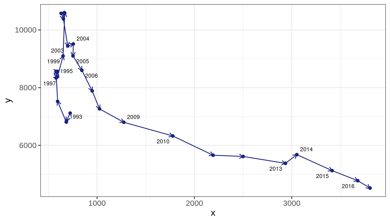
6 1996 593 8565Visualization
# Connected Scatterplot
connected_scatterplot <- function(data, x, y, label, label_ratio, line_color, arrow_size, label_size) {

  draw_data <- data.frame(
    x = data[[x]],
    y = data[[y]],
    label = data[[label]]
  )

  add_label_data <- draw_data %>% sample_frac(label_ratio)
  rm(data)

  p <- ggplot(draw_data, aes(x = x, y = y, label = label)) +
    geom_point(color = line_color) +
    geom_text_repel(data = add_label_data, size = label_size) +
    geom_segment(
      color = line_color,
      aes(
        xend = c(tail(x, n = -1), NA),
        yend = c(tail(y, n = -1), NA)
      ),
      arrow = arrow(length = unit(arrow_size, "mm"))
    )

  return(p)
}

p <- connected_scatterplot(
  data = if (exists("data") && is.data.frame(data)) data else "",
  x = "Alice",
  y = "Anna",
  label = "year",
  label_ratio = 0.5,
  line_color = "#1A237E",
  arrow_size = 2,
  label_size = 2.5
) +
  theme_bw() +
  theme(text = element_text(family = "Arial"),
        plot.title = element_text(size = 12,hjust = 0.5),
        axis.title = element_text(size = 12),
        axis.text = element_text(size = 10),
        axis.text.x = element_text(angle = 0, hjust = 0.5,vjust = 1),
        legend.position = "right",
        legend.direction = "vertical",
        legend.title = element_text(size = 10),
        legend.text = element_text(size = 10))

p