Regression Analysis Table

The regression analysis table is used to display the results of the regression model. It provides statistical information about the variables in the model and helps explain the relationship between the variables.

Example

The figure below shows a regression analysis based on the pbc dataset built into the survival package. The figure uses the Cox proportional hazards model and generalized linear regression model to explore the effects of serum protein, sex, and age on survival.

Setup

• System Requirements: Cross-platform (Linux/MacOS/Windows)

• Programming language: R

• Dependent packages: survival, gtsummary, dplyr, datawizard

# Installing packages
if (!requireNamespace("survival", quietly = TRUE)) {
  install.packages("survival")
}
if (!requireNamespace("gtsummary", quietly = TRUE)) {
  install.packages("gtsummary")
}
if (!requireNamespace("dplyr", quietly = TRUE)) {
  install.packages("dplyr")
}
if (!requireNamespace("datawizard", quietly = TRUE)) {
  install.packages("datawizard")
}
if (!requireNamespace("broom.helpers", quietly = TRUE)) {
  install.packages("broom.helpers")
}

# Load packages
library(survival)
library(gtsummary)
library(dplyr)
library(datawizard)
library(broom.helpers)

Data Preparation

The pbc dataset, built into the survival R package, contains information on 418 patients with primary biliary cirrhosis (PBC) who had received ursodeoxycholic acid (UDCA) treatment at or before the start of the study. The pbc dataset records clinical information such as survival time, survival status, treatment method, age, sex, albumin level, and hepatomegaly.

df <- pbc %>%
  filter(status != 1) %>%
  mutate(status = ifelse(status == 2, 1, 0)) %>%
  select(2:13) %>%
  na.omit() %>% 
  # Divide `albumin` into 3 groups
  mutate(albumin3cat = categorize(albumin, split = "quantile", n_groups = 3))

head(df[,1:6])

  time status trt      age sex ascites
1  400      1   1 58.76523   f       1
2 4500      0   1 56.44627   f       0
3 1012      1   1 70.07255   m       0
4 1925      1   1 54.74059   f       0
5 2503      1   2 66.25873   f       0
6 1832      0   2 55.53457   f       0

Visualization

1. Basic regression analysis table

# Basic regression analysis table
t1 <- coxph(Surv(time, status) ~ albumin + sex + age,
  data = df
) %>%
  tbl_regression()

t1

Characteristic	log(HR)	95% CI	p-value
albumin	-1.7	-2.1, -1.2	<0.001
sex
m	—	—
f	-0.56	-1.1, -0.06	0.027
age	0.03	0.01, 0.05	0.004
Abbreviations: CI = Confidence Interval, HR = Hazard Ratio

Figure 1: Basic regression analysis table

This table is a basic regression analysis table. The Cox proportional hazard model is called by coxph() and the results of the regression analysis are tabulated using tbl_regression().

2. tbl_regression() parameter settings

# tbl_regression() parameter settings
t1 <- coxph(Surv(time, status) ~ albumin + sex + age,
  data = df
) %>%
  # parameter settings
  tbl_regression(
    conf.level = 0.90,
    exponentiate = TRUE,
    include = c("sex", "albumin"),
    show_single_row = sex,
    label = list(sex ~ "sex as categorical")
  )

t1

Characteristic	HR	90% CI	p-value
sex as categorical	0.57	0.37, 0.87	0.027
albumin	0.19	0.13, 0.28	<0.001
Abbreviations: CI = Confidence Interval, HR = Hazard Ratio

Figure 2: tbl_regression() parameter settings

There are many parameter settings in the table tbl_regression(), which can change the confidence interval, row names and other information of the table.

Tip

Important parameter: tbl_regression

• conf.level: Determines the confidence level for the regression analysis. The default value of 0.95 indicates a 95% confidence interval.

• exponentiate: Whether to exponentiate the HR values. The default column is log(HR) values.

• include: Which independent variables (rows) are included in the statistical table.

• show_single_row: Applies to binary variables and does not display the control group.

• label: Changes the name (row name) of the independent variable.

3. Add global-p

# Add global-p
df$albumin3cat=as.factor(df$albumin3cat)

t1 <- coxph(Surv(time, status) ~ albumin3cat + sex + age,
            data = df) %>%
  tbl_regression()  %>%
  add_global_p()

t1

Characteristic	log(HR)	95% CI	p-value
albumin3cat			<0.001
1	—	—
2	-0.72	-1.2, -0.27
3	-1.3	-1.7, -0.77
sex			0.073
m	—	—
f	-0.48	-0.98, 0.02
age	0.03	0.01, 0.05	<0.001
Abbreviations: CI = Confidence Interval, HR = Hazard Ratio

Figure 3: Add global-p

This table adds global P values via add_global_p().

4. Add q-value

# Add q-value
t1 <- coxph(Surv(time, status) ~ albumin + sex + age,
  data = df
) %>%
  tbl_regression() %>%
  # Add a q-value column
  add_q()

t1

Characteristic	log(HR)	95% CI	p-value	q-value1
albumin	-1.7	-2.1, -1.2	<0.001	<0.001
sex
m	—	—
f	-0.56	-1.1, -0.06	0.027	0.027
age	0.03	0.01, 0.05	0.004	0.006
Abbreviations: CI = Confidence Interval, HR = Hazard Ratio
1 False discovery rate correction for multiple testing

Figure 4: Add q-value

The table adds a q-value column via add_q().

5. Merge columns

# Merge columns
t1 <- coxph(Surv(time, status) ~ albumin3cat + sex + age,
            data = df) %>%
  tbl_regression()  %>%
  # Modify the header name
  modify_header(p.value = "**P**",estimate="**log(HR) (CI)**") %>%
  # Combine the score column and the CI column and apply to rows where the score is not NA
  modify_column_merge(
    pattern = "{estimate} ({conf.low}, {conf.high})",
    rows = !is.na(estimate)
  )

t1

Characteristic	log(HR) (CI)	P
albumin3cat
1	—
2	-0.72 (-1.2, -0.27)	0.002
3	-1.3 (-1.7, -0.77)	<0.001
sex
m	—
f	-0.48 (-0.98, 0.02)	0.062
age	0.03 (0.01, 0.05)	<0.001
Abbreviations: CI = Confidence Interval, HR = Hazard Ratio

Figure 5: Merge columns

This table merges the score column and the CI column, which is a common form. The table header is appropriately modified after the merger.

Tip

Important Functions modify_header / modify_column_merge:

modify_header:modify_header() can be used to modify the header name. label represents the variable column, p.value represents the P-value column, ci represents the confidence interval column, estimate represents the score column, conf.low represents the lower confidence interval, and conf.high represents the upper confidence interval.

modify_column_merge: The pattern parameter specifies the pattern of columns to be merged, and the rows parameter specifies the rows to apply the merge to.

6. Model integration

Model horizontal integration合

# Model horizontal integration
t1 <- coxph(Surv(time, status) ~ albumin + sex + age,
  data = df
) %>%
  tbl_regression()
t2 <- glm(time ~ albumin + sex + age,
  data = df
) %>%
  tbl_regression()
# t1, t2 model integration
t3 <- tbl_merge(
  tbls = list(t1, t2),
  tab_spanner = c("**Cox Model**", "**GLM Model**")
)

t3

Characteristic	Cox Model			GLM Model
	log(HR)	95% CI	p-value	Beta	95% CI	p-value
albumin	-1.7	-2.1, -1.2	<0.001	1,128	813, 1,442	<0.001
sex
m	—	—		—	—
f	-0.56	-1.1, -0.06	0.027	34	-360, 428	0.9
age	0.03	0.01, 0.05	0.004	-7.7	-20, 4.9	0.2
Abbreviations: CI = Confidence Interval, HR = Hazard Ratio

Figure 6: Model horizontal integration

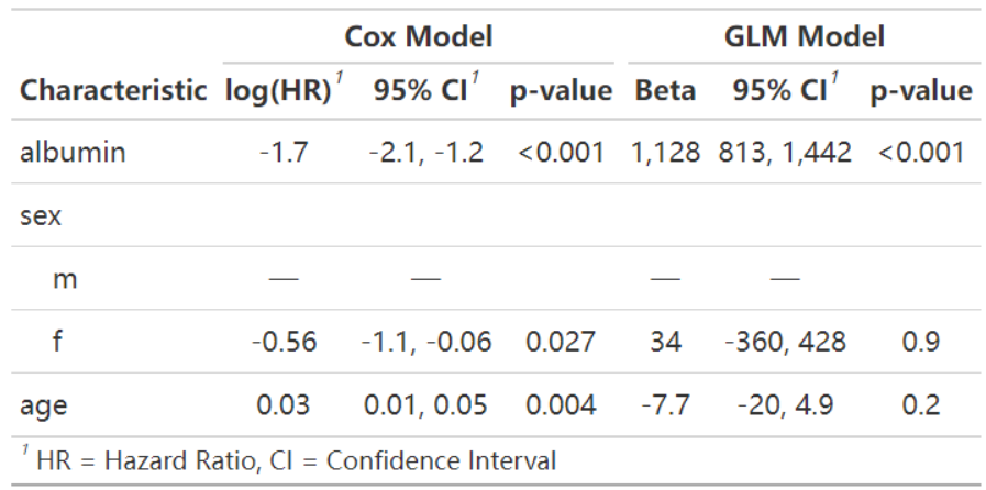
This table uses tbl_merge to horizontally integrate the results of the Cox proportional hazards model and the generalized linear regression model for patients with pdb.

Model vertical integration

# Model vertical integration
t1 <- coxph(Surv(time, status) ~ albumin + sex + age,
  data = df[df$hepato==0,]
) %>%
  tbl_regression()

t2 <- coxph(Surv(time, status) ~ albumin + sex + age,
  data = df[df$hepato==1,]
) %>%
  tbl_regression()

tbl_stack(list(t1, t2), group_header = c("Patients without hepato", "Patients with hepato"))

Characteristic	log(HR)	95% CI	p-value
Patients without hepato
albumin	-1.4	-2.3, -0.47	0.003
sex
m	—	—
f	-1.1	-1.9, -0.36	0.004
age	0.06	0.03, 0.09	<0.001
Patients with hepato
albumin	-1.4	-2.0, -0.87	<0.001
sex
m	—	—
f	-0.29	-0.97, 0.38	0.4
age	0.01	-0.01, 0.04	0.3
Abbreviations: CI = Confidence Interval, HR = Hazard Ratio

Figure 7: Model vertical integration

This table uses tbl_stack to longitudinally integrate the results of the Cox proportional hazards model for the two groups of pdb patients with and without hepato.

Application

Figure 8: Regression Analysis Table

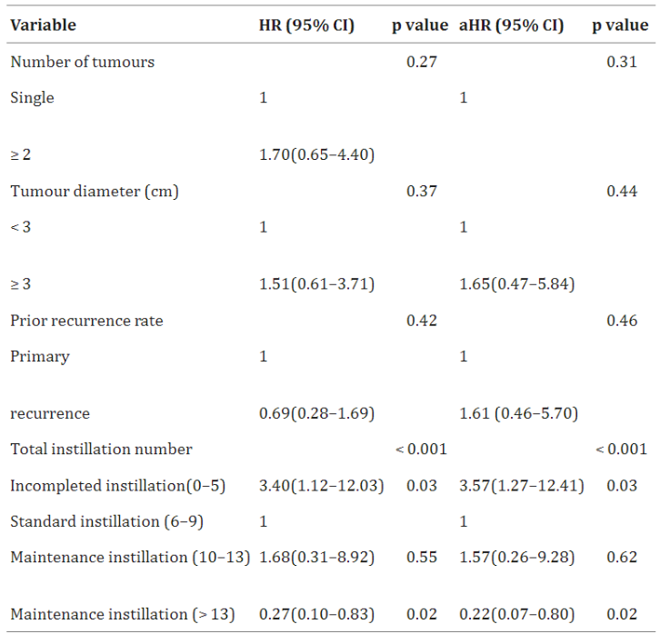
Univariate and multivariate Cox regression analyses were performed to assess 3-year tumor recurrence in patients with intermediate-risk NMIBC. [1]

Figure 9: Regression Analysis Table

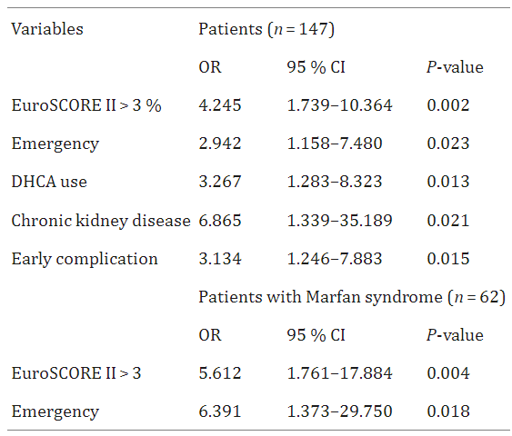
This regression analysis table shows the independent predictors of late total mortality in multivariable Cox regression analysis. [2]

Reference

[1] CHEN J X, HUANG W T, ZHANG Q Y, et al. The optimal intravesical maintenance chemotherapy scheme for the intermediate-risk group non-muscle-invasive bladder cancer[J]. BMC Cancer, 2023,23(1): 1018.

[2] BENKE K, ÁGG B, SZABÓ L, et al. Bentall procedure: quarter century of clinical experiences of a single surgeon[J]. J Cardiothorac Surg, 2016,11: 19.