China Map

Authors

[Editor] Hu Zheng;

[Contributors]

Modified

2026-09-13

🤖 AI Skill — Download the Bizard unified skill for your AI assistant ⬇️ Download Skill ZIP

Note

Hiplot website

This page is the tutorial for source code version of the Hiplot China Map plugin. You can also use the Hiplot website to achieve no code ploting. For more information please see the following link:

https://hiplot.cn/basic/map-china?lang=en

Setup

System Requirements: Cross-platform (Linux/MacOS/Windows)
Programming language: R
Dependent packages: data.table; jsonlite; ggplot2; RColorBrewer

# Install packages
if (!requireNamespace("data.table", quietly = TRUE)) {
  install.packages("data.table")
}
if (!requireNamespace("jsonlite", quietly = TRUE)) {
  install.packages("jsonlite")
}
if (!requireNamespace("ggplot2", quietly = TRUE)) {
  install.packages("ggplot2")
}
if (!requireNamespace("RColorBrewer", quietly = TRUE)) {
  install.packages("RColorBrewer")
}

# Load packages
library(data.table)
library(jsonlite)
library(ggplot2)
library(RColorBrewer)

sessioninfo::session_info("attached")

─ Session info ───────────────────────────────────────────────────────────────
 setting  value
 version  R version 4.6.0 (2026-04-24)
 os       Ubuntu 24.04.4 LTS
 system   x86_64, linux-gnu
 ui       X11
 language (EN)
 collate  C.UTF-8
 ctype    C.UTF-8
 tz       UTC
 date     2026-05-09
 pandoc   3.1.3 @ /usr/bin/ (via rmarkdown)
 quarto   1.9.37 @ /usr/local/bin/quarto

─ Packages ───────────────────────────────────────────────────────────────────
 package      * version    date (UTC) lib source
 data.table   * 1.18.4     2026-05-06 [1] RSPM
 ggplot2      * 4.0.3.9000 2026-05-04 [1] Github (tidyverse/ggplot2@6870419)
 jsonlite     * 2.0.0      2025-03-27 [1] RSPM
 RColorBrewer * 1.1-3      2022-04-03 [1] RSPM

 [1] /home/runner/work/_temp/Library
 [2] /opt/R/4.6.0/lib/R/site-library
 [3] /opt/R/4.6.0/lib/R/library
 * ── Packages attached to the search path.

──────────────────────────────────────────────────────────────────────────────

Data Preparation

# Load data
data <- data.table::fread(jsonlite::read_json("https://hiplot.cn/ui/basic/map-china/data.json")$exampleData$textarea[[1]])
data <- as.data.frame(data)
dt_map <- readRDS(url("https://download.hiplot.cn/ui/basic/map-china/china.rds"))

# Convert data structure
dt_map$Value <- data$value[match(dt_map$FCNAME, data$name)]

# View data
head(data)

    name value
1 安徽省  6118
2 福建省  3581
3 甘肃省  2617
4 广东省  9449
5 贵州省  3762
6 海南省   845

Visualization

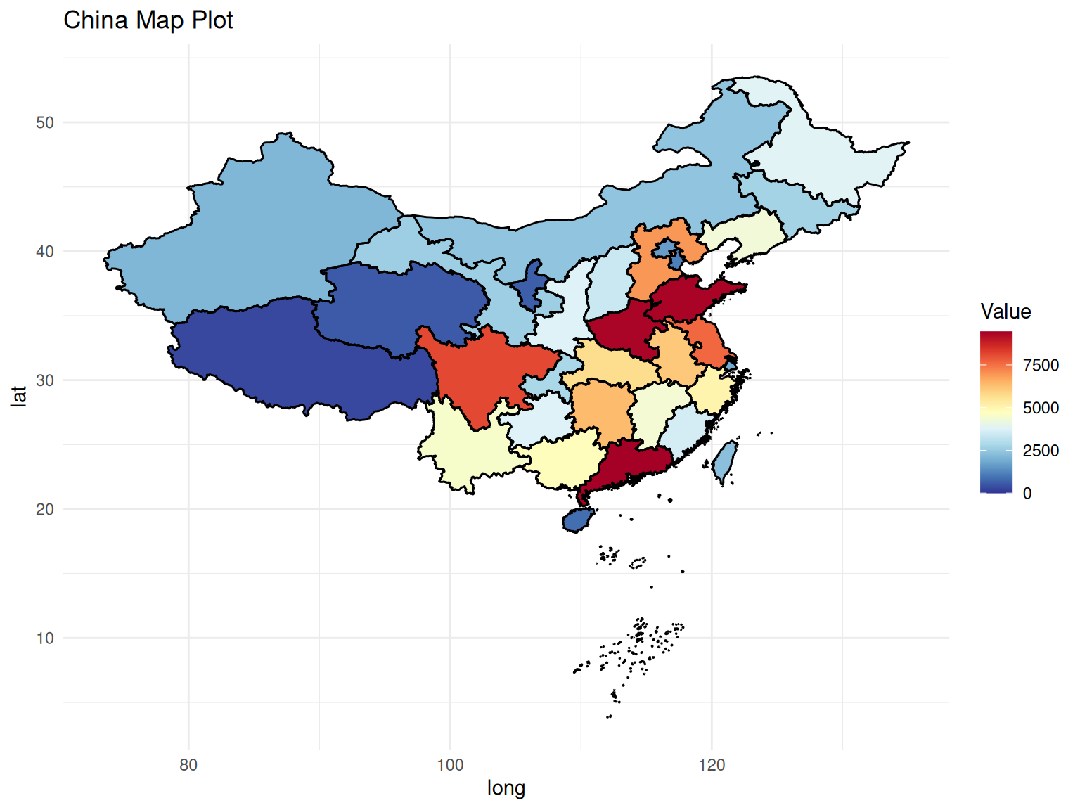
# China Map
p <- ggplot(dt_map, aes(x = long, y = lat, group = group, fill = Value)) +
  labs(fill = "Value") +
  geom_polygon() +
  geom_path() +
  coord_fixed() +
  scale_fill_gradientn(
    colours = colorRampPalette(rev(brewer.pal(11,"RdYlBu")))(500),
    na.value = "grey10",
    limits = c(0, max(dt_map$Value) * 1.2)) +
    ggtitle("China Map Plot") +
  theme_minimal()

p