# Installing necessary packages
if (!requireNamespace("rms", quietly = TRUE)) {
  install.packages("rms")
}

# Load packages
library(survival)
library(dplyr)
library(ggplot2)
library(rms)Calibration Curve
A calibration curve assesses the accuracy of a prediction model: among patients predicted to have a given risk, how often does the event actually occur? A perfectly calibrated model lies on the 45° line of a plot of observed versus predicted probabilities. Discrimination (see the ROC curve tutorial) and calibration answer different questions — a model can rank patients well yet systematically over- or under-estimate absolute risks [1]. Together with decision curve analysis, calibration is part of the standard evaluation suite of clinical prediction models.
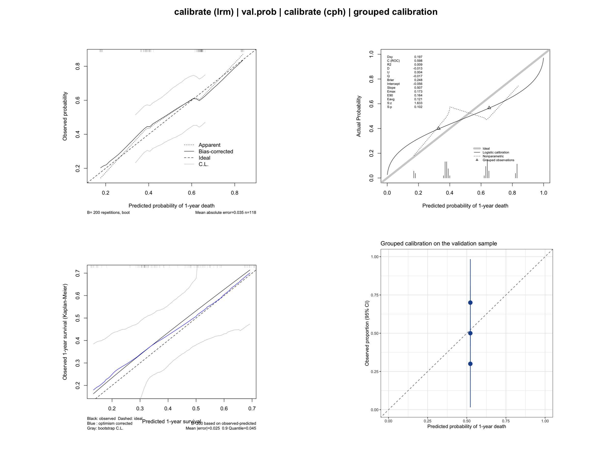
This tutorial covers four calibration workflows in R (rms package):
- Logistic-model calibration with bootstrap smoothing (
calibrate); - External-style validation of predicted probabilities (
val.prob); - Cox-model calibration of predicted survival at a fixed horizon;
- A ggplot2 version with grouped observed-versus-predicted rates.
Example
Setup
System Requirements: Cross-platform (Linux/MacOS/Windows)
Programming language: R
Dependent packages:
survival;dplyr;rms;ggplot2
sessioninfo::session_info("attached")─ Session info ───────────────────────────────────────────────────────────────
setting value
version R version 4.6.1 (2026-06-24)
os Ubuntu 24.04.5 LTS
system x86_64, linux-gnu
ui X11
language (EN)
collate C.UTF-8
ctype C.UTF-8
tz UTC
date 2026-10-29
pandoc 3.1.3 @ /usr/bin/ (via rmarkdown)
quarto 1.10.19 @ /usr/local/bin/quarto
─ Packages ───────────────────────────────────────────────────────────────────
! package * version date (UTC) lib source
P dplyr * 1.2.1 2026-04-03 [?] RSPM
P ggplot2 * 4.0.3.9000 2026-10-26 [?] Github (tidyverse/ggplot2@b638d65)
P Hmisc * 5.3-0 2026-09-06 [?] RSPM
P rms * 8.1-1 2026-02-18 [?] RSPM
survival * 3.8-6 2026-01-16 [3] CRAN (R 4.6.1)
[1] /home/runner/.cache/R/renv/library/Bizard-5140bdc6/linux-ubuntu-noble/R-4.6/x86_64-pc-linux-gnu
[2] /home/runner/work/_temp/Library
[3] /opt/R/4.6.1/lib/R/library
* ── Packages attached to the search path.
P ── Loaded and on-disk path mismatch.
──────────────────────────────────────────────────────────────────────────────Data Preparation
We again use the lung data set from the survival package (North Central Cancer Treatment Group lung cancer trial) [2], with death within one year as the binary endpoint for the logistic models and overall survival for the Cox model. The data are split into a training and a validation subsample to demonstrate val.prob().
data(lung, package = "survival")

set.seed(2026)
lung2 <- lung %>%
  filter(complete.cases(age, sex, ph.ecog, ph.karno, pat.karno, meal.cal, wt.loss)) %>%
  mutate(y1y = as.integer(time < 365 & status == 2))  # death within 365 days
  # Caveat: patients censored before day 365 are counted as non-events.

idx <- sample(seq_len(nrow(lung2)), size = round(0.7 * nrow(lung2)))
train <- lung2[idx, ]
valid <- lung2[-idx, ]

cat("Train:", nrow(train), " Valid:", nrow(valid),
    " Events (train):", sum(train$y1y), "\n")
Train: 118 Valid: 50 Events (train): 63 dd <- datadist(lung2) # datadist based on the full data
options(datadist = "dd")Visualization
1. Logistic-Model Calibration with Bootstrap Smoothing
calibrate() on a lrm fit uses bootstrap-corrected estimates of the predicted-versus-observed curve, which is less noisy than a raw grouping of a single sample [3].
lrm_fit <- lrm(y1y ~ age + sex + ph.ecog, data = train, x = TRUE, y = TRUE)
set.seed(2026)  # keep the bootstrap calibration reproducible across renders
cal_lrm <- calibrate(lrm_fit, method = "boot", B = 200)
plot(cal_lrm, xlab = "Predicted probability of 1-year death",
     ylab = "Observed probability")
n=118   Mean absolute error=0.035   Mean squared error=0.00146
0.9 Quantile of absolute error=0.054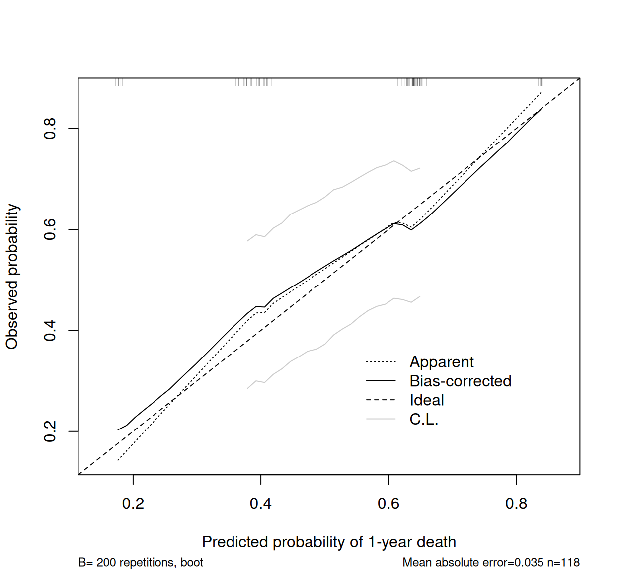
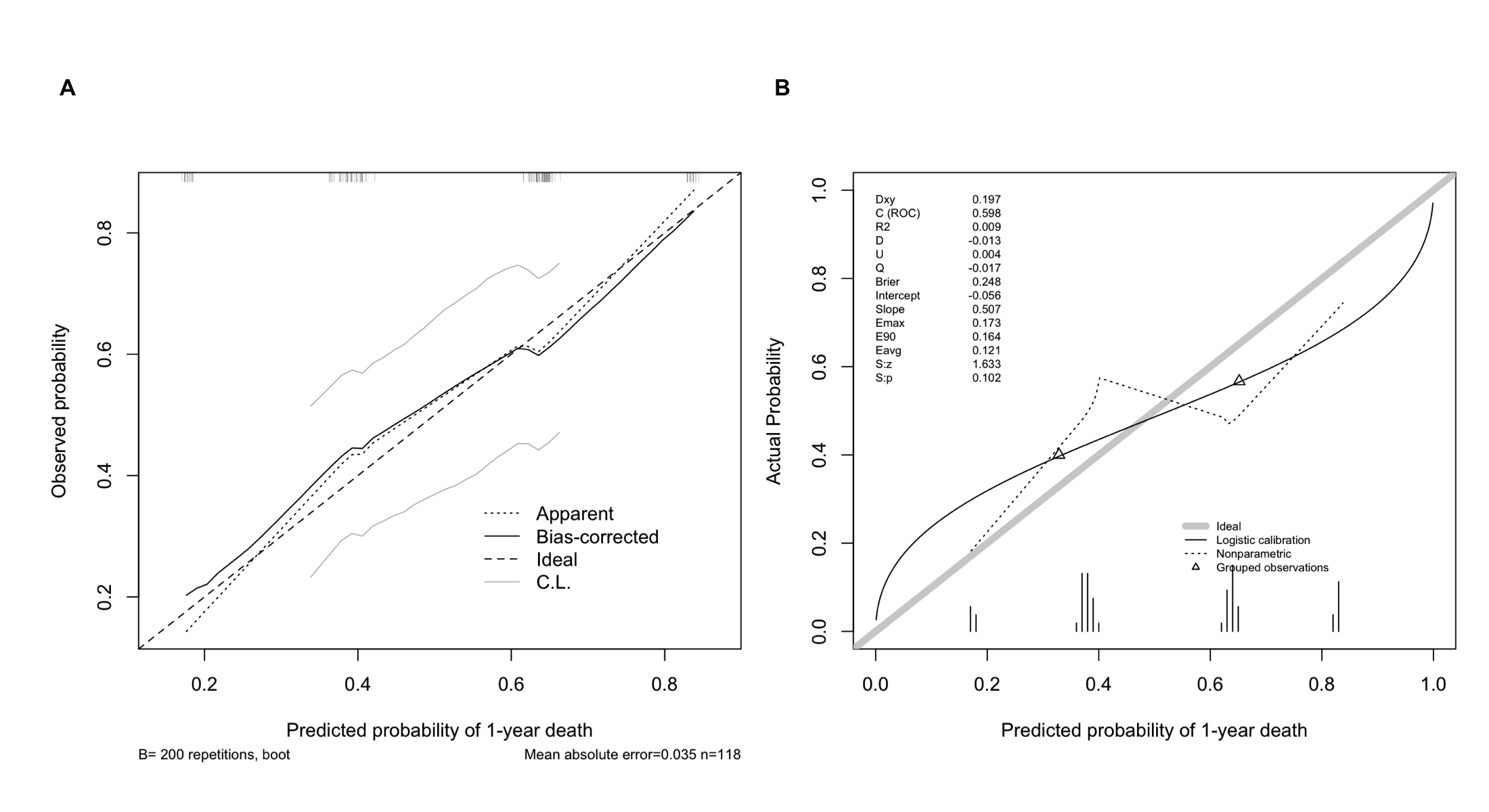
The “apparent” line is the in-sample fit; the “bias-corrected” line adjusts for overfitting and is the one to report. A slope below 1 indicates predictions that are too extreme (overfit).
2. Validating Predicted Probabilities with val.prob
val.prob() takes predicted probabilities and the binary outcome of an independent sample and reports the calibration intercept, slope, discrimination (C-index = AUC), Brier score and more.
pred_valid <- predict(lrm_fit, newdata = valid, type = "fitted")
val.prob(pred_valid, valid$y1y,
         m = 20, cex = 0.6,   # groups of 20 observations for the plotted points
         xlab = "Predicted probability of 1-year death")
Dxy C (ROC) R2 D D:Chi-sq D:p
0.196800000 0.598400000 0.008968521 -0.013250885 0.337455734 0.561301515
U U:Chi-sq U:p Q Brier Intercept
0.004118724 2.205936208 0.331884552 -0.017369609 0.247916126 -0.056285313
Slope Emax E90 Eavg S:z S:p
0.507292141 0.172801139 0.163772477 0.121254444 1.633283299 0.102409428 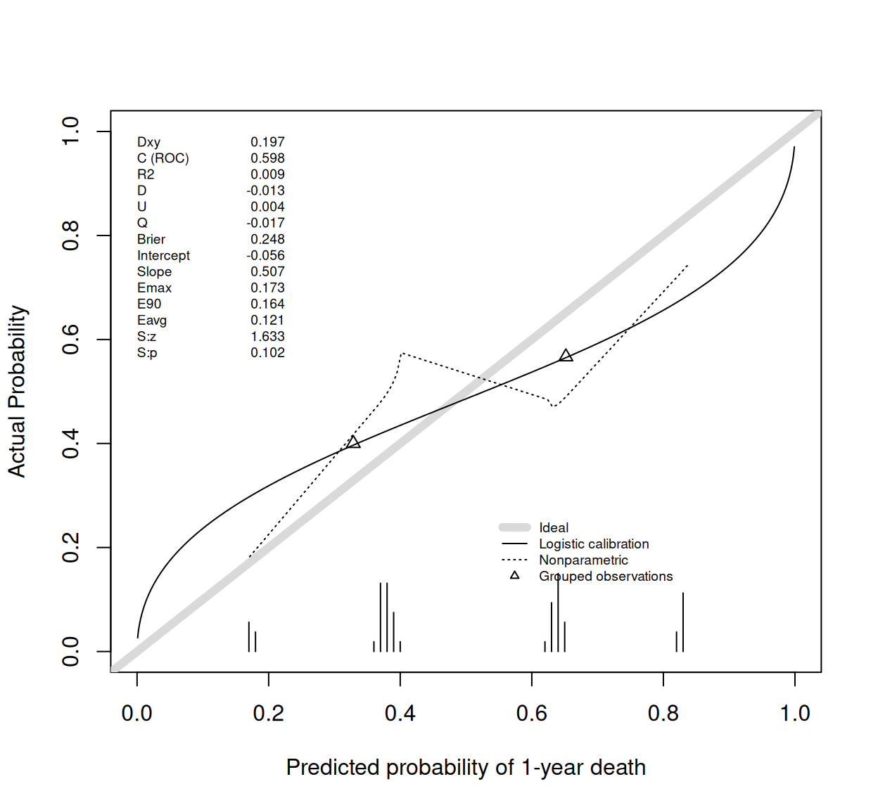
The thick grey diagonal is ideal calibration; the triangles mark the grouped observed rates (20 per group). The printed statistics include the calibration intercept (ideally 0) and calibration slope (ideally 1).
3. Cox-Model Calibration of Survival Probabilities
For survival models, calibration is assessed at a fixed horizon: the predicted probability of surviving one year is compared with the Kaplan-Meier observed proportion [3].
cph_fit <- cph(Surv(time, status) ~ age + sex + ph.ecog,
               data = train, x = TRUE, y = TRUE, surv = TRUE, time.inc = 365)
set.seed(2026)
cal_cph <- calibrate(cph_fit, u = 365, method = "boot", B = 200, m = 40)
Using Cox survival estimates at 365 Daysplot(cal_cph, xlab = "Predicted 1-year survival",
ylab = "Observed 1-year survival (Kaplan-Meier)")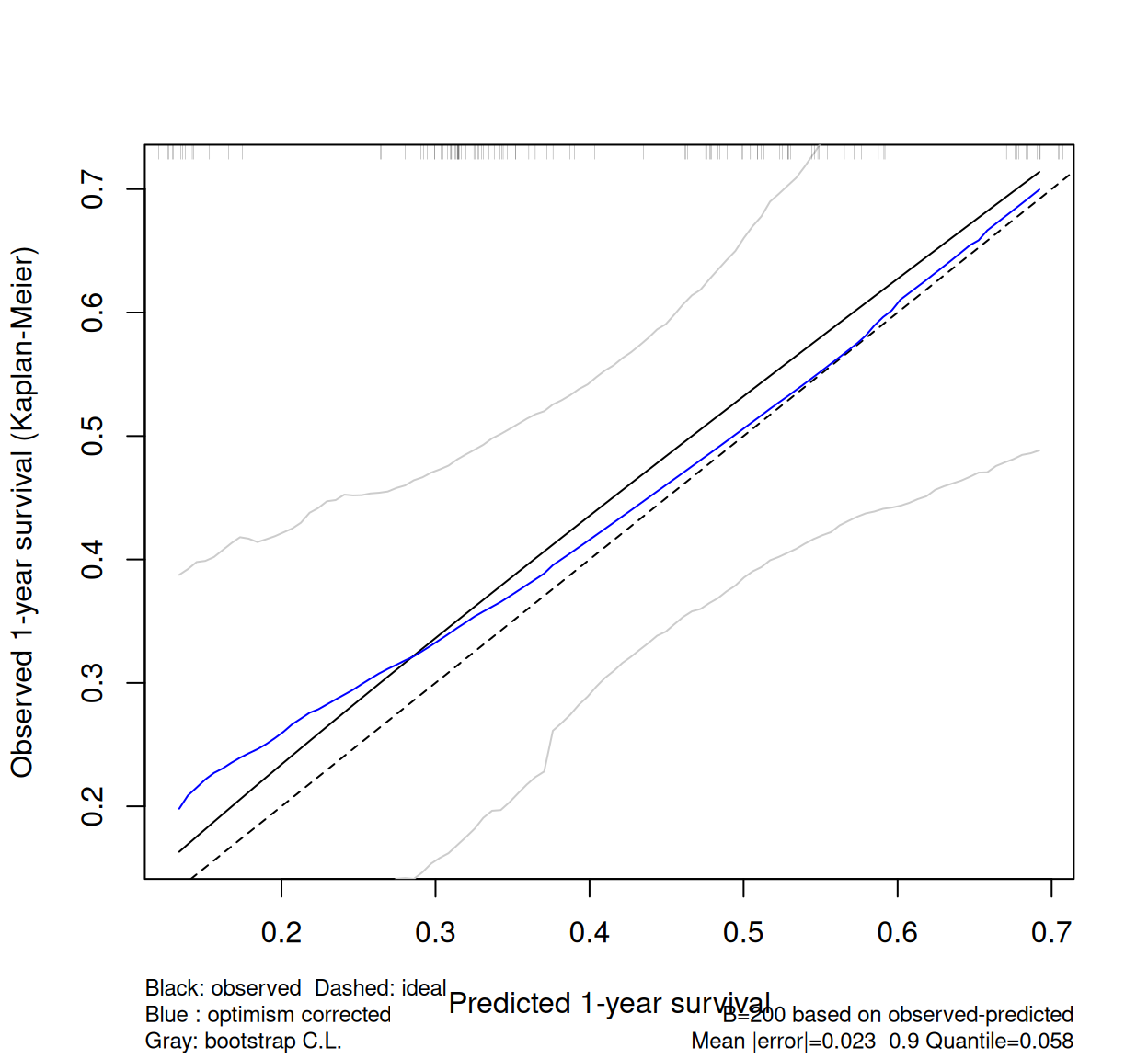
u = 365 must match time.inc in the cph call, and m controls the number of observations per group used to estimate the curve.
4. A ggplot2 Version with Grouped Calibration Points
valid$pred_valid <- pred_valid  # needed so each group uses its own predictions

grouped <- valid %>%
  mutate(pred_group = ntile(pred_valid, n = 5)) %>%
  group_by(pred_group) %>%
  summarise(mean_pred = mean(pred_valid),
            obs_rate = mean(y1y),
            se = sqrt(obs_rate * (1 - obs_rate) / n()),
            n = n(),
            .groups = "drop")

ggplot(grouped, aes(mean_pred, obs_rate)) +
  geom_abline(slope = 1, intercept = 0, linetype = "dashed", color = "grey50") +
  geom_pointrange(aes(ymin = pmax(obs_rate - 1.96 * se, 0),
                      ymax = pmin(obs_rate + 1.96 * se, 1)),
                  color = "#2166AC", size = 0.8) +
  coord_cartesian(xlim = c(0, 1), ylim = c(0, 1)) +
  labs(x = "Predicted probability of 1-year death",
       y = "Observed proportion (95% CI)",
       title = "Grouped calibration on the validation sample") +
  theme_bw()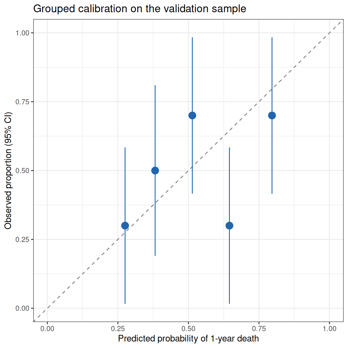
This transparent construction — bucket predictions, compare observed event rates — is exactly what grouped calibration curves show, and makes the sample size behind each point visible. Note the wide intervals: calibration assessment needs large samples.
Application
Calibration curves are reported alongside nomograms in prediction-model papers, typically as “training set + validation set” pairs. The panel below mirrors that layout with this tutorial’s outputs: (A) bootstrap-corrected calibration on the training sample and (B) independent-sample validation with val.prob.
Reference
[1] Van Calster B, McLernon DJ, van Smeden M, et al. Calibration: the Achilles heel of predictive analytics. BMC Med. 2019;17(1):230. doi:10.1186/s12916-019-1466-7
[2] Loprinzi CL, Laurie JA, Wieand HS, et al. Prospective evaluation of prognostic variables from patient-completed questionnaires. North Central Cancer Treatment Group. J Clin Oncol. 1994;12(3):601-607. doi:10.1200/JCO.1994.12.3.601
[3] Harrell FE Jr. Regression Modeling Strategies: With Applications to Linear Models, Logistic and Ordinal Regression, and Survival Analysis. 2nd ed. Springer; 2015. doi:10.1007/978-3-319-19425-7
[4] Collins GS, Reitsma JB, Altman DG, Moons KGM. Transparent Reporting of a multivariable prediction model for Individual Prognosis Or Diagnosis (TRIPOD). BMJ. 2015;350:g7594. doi:10.1136/bmj.g7594