Joint & Pair Plot (Python)

🤖 AI Skill — Download the Bizard unified skill for your AI assistant ⬇️ Download Skill ZIP

🔌 MCP Server — Let AI agents (Claude Code, Cursor, …) query Bizard live: claude mcp add bizard -- npx @openbiox/bizard-mcp — or the free hosted instance (no install, faster from mainland China): claude mcp add --transport http bizard http://biotree.top:38123/bizard-mcp/mcp 📖 MCP Docs

📖 Cite Bizard — if Bizard helps your research, please cite: Li, K., Zheng, H., Huang, K., et al. (2026). Bizard: A Community-Driven Platform for Accelerating and Enhancing Biomedical Data Visualization. iMetaMed, e70038. 🔗 DOI / BibTeX

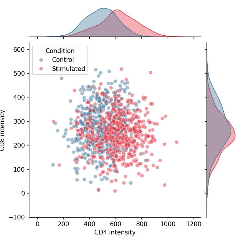
A joint plot pairs a bivariate display (scatter or KDE) with the marginal distributions of each variable along the axes; a pair plot extends this idea to every pairwise combination of variables in a matrix. In biomedical research they are the standard first look at how measurements co-vary — marker-to-marker correlations, biomarker panels, or multi-assay quality metrics. seaborn provides both through jointplot and pairplot.

Example

Setup

• System Requirements: Cross-platform (Linux/MacOS/Windows)
• Programming Language: Python
• Dependencies: matplotlib, seaborn, pandas, numpy

import matplotlib.pyplot as plt
import seaborn as sns
import pandas as pd
import numpy as np

Data Preparation

We simulate a two-marker flow panel across stimulated and control cells, and load the classic iris measurements for the multi-variable pair plot.

np.random.seed(61)

n = 500
flow = pd.DataFrame({
    'CD4': np.concatenate([np.random.normal(500, 120, n),
                           np.random.normal(620, 140, n)]),
    'CD8': np.concatenate([np.random.normal(280, 90, n),
                           np.random.normal(250, 85, n)]),
    'Condition': np.repeat(['Control', 'Stimulated'], n)
})

Visualization

Joint Plot with Scatter and Marginals

seaborn.jointplot draws the central scatter plus marginal histograms; hue splits both the joint and marginal layers by condition.

g = sns.jointplot(data=flow, x='CD4', y='CD8', hue='Condition',
                  palette={'Control': '#457b9d', 'Stimulated': '#e63946'},
                  alpha=0.5, height=5.5, marginal_kws=dict(fill=True, alpha=0.4))
g.set_axis_labels('CD4 intensity', 'CD8 intensity')
plt.show()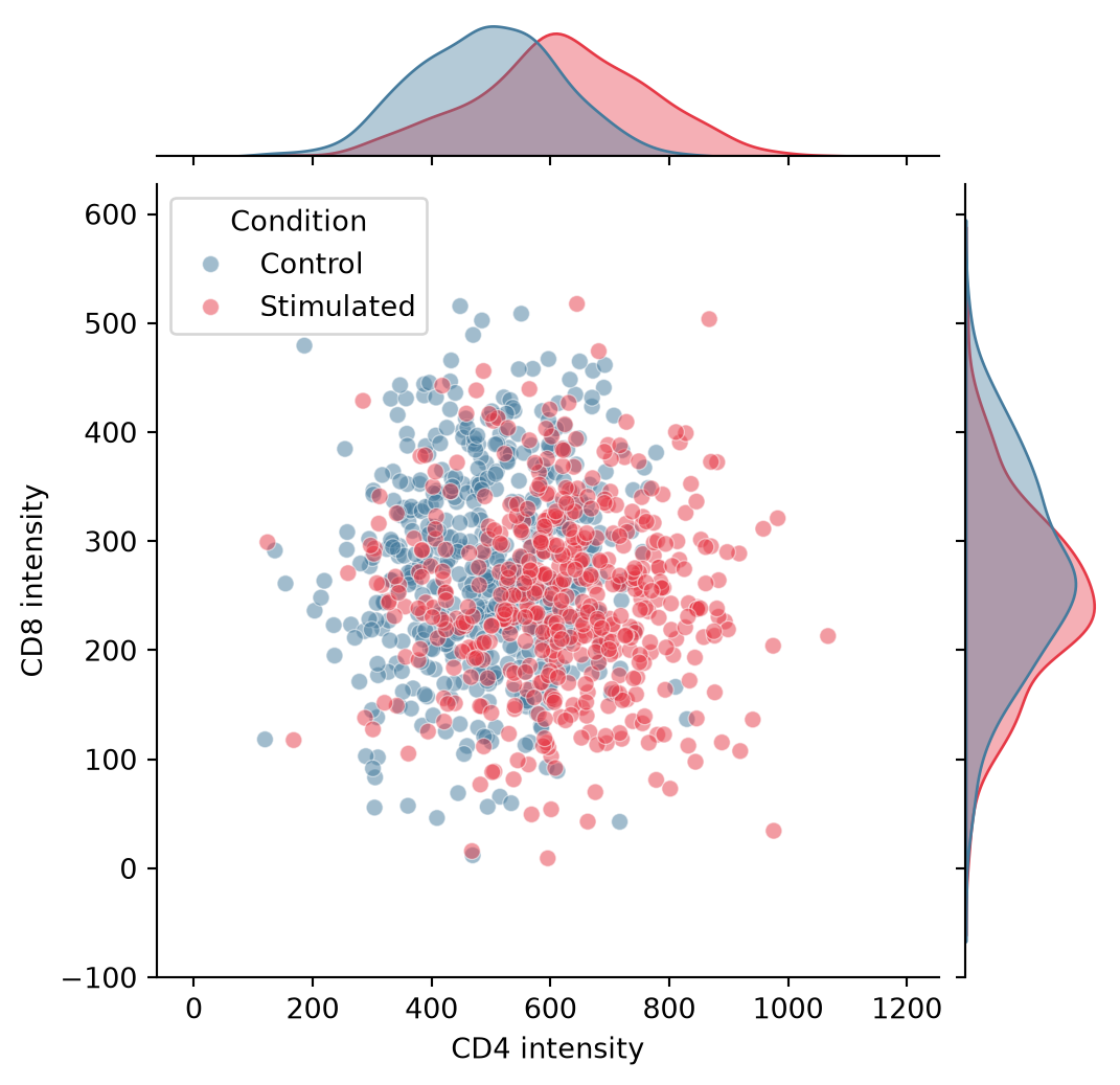

Figure 1: Joint plot of CD4 vs CD8 with marginal distributions

Joint Plot with KDE and Hexbin

For dense samples, switch the central layer: kind='kde' contours the bivariate density, while kind='hex' bins millions of points without overplotting.

g = sns.jointplot(data=flow, x='CD4', y='CD8', hue='Condition',
                  kind='kde',
                  palette={'Control': '#457b9d', 'Stimulated': '#e63946'},
                  height=5.5, marginal_kws=dict(fill=True, alpha=0.4),
                  joint_kws=dict(alpha=0.7))
g.set_axis_labels('CD4 intensity', 'CD8 intensity')
plt.show()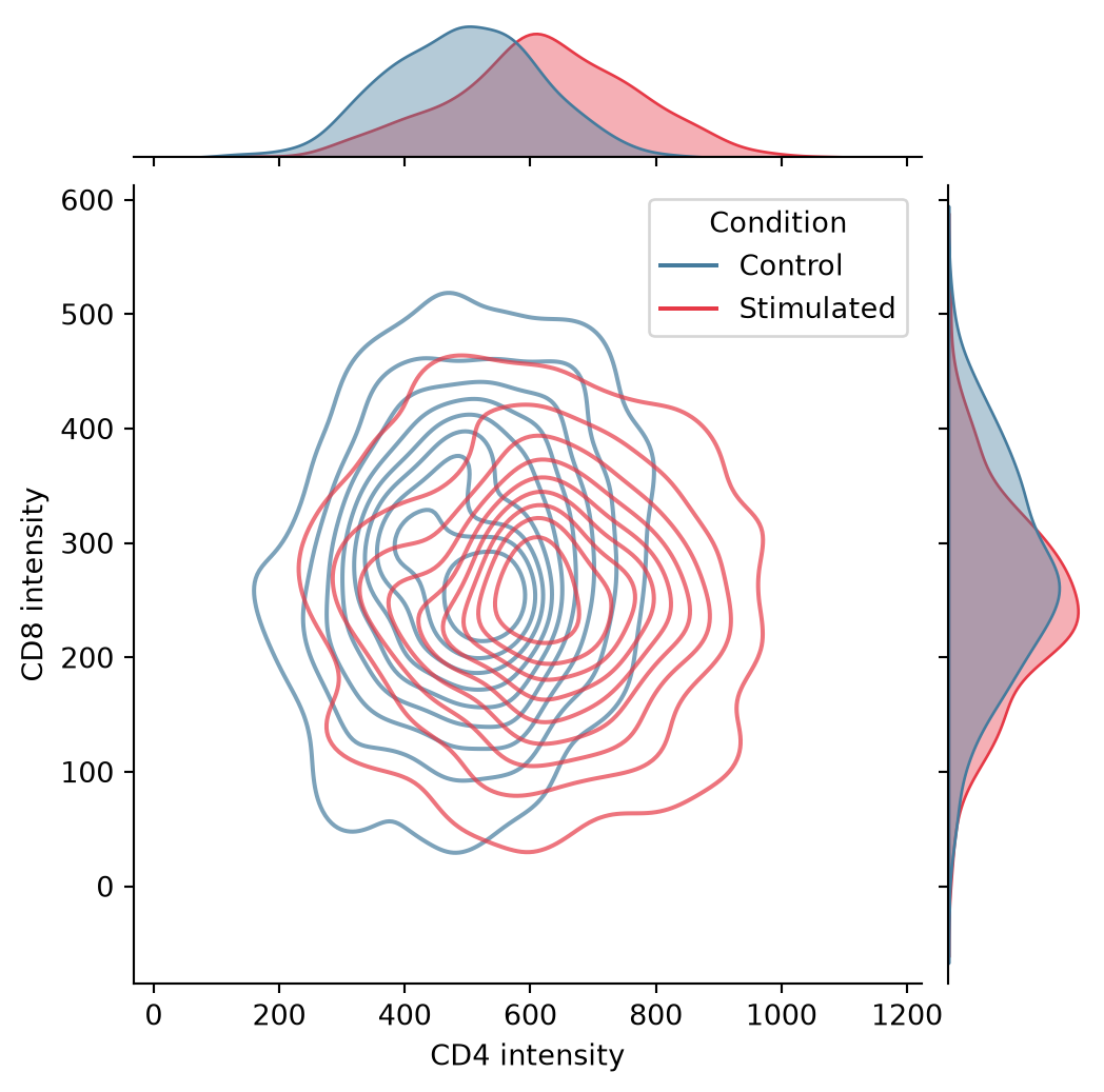

Figure 2: Joint plot with KDE contours and density marginals

Pair Plot Matrix

seaborn.pairplot builds the full scatterplot matrix with diagonals showing each variable’s distribution; corner=True removes the redundant upper triangle.

iris = sns.load_dataset('iris')
g = sns.pairplot(iris, hue='species', corner=True,
                 palette='Set2',
                 plot_kws=dict(alpha=0.6, s=20),
                 diag_kws=dict(fill=True, alpha=0.4))
plt.show()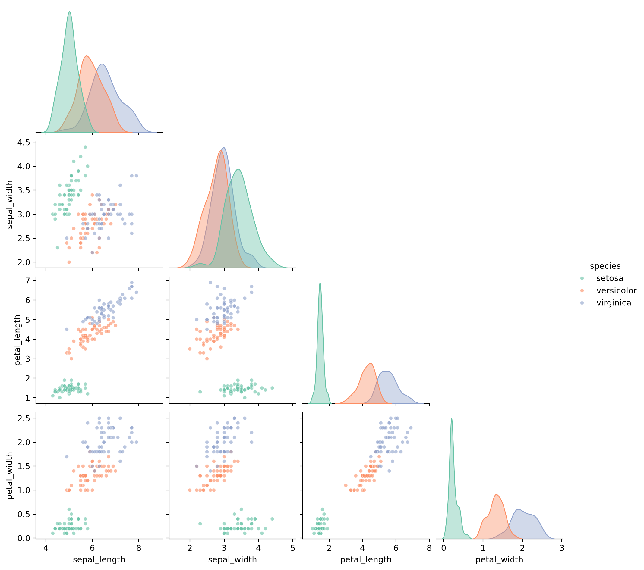

Figure 3: Pair plot of iris measurements by species (corner layout)

References

1. Waskom, M. L. (2021). seaborn: statistical data visualization. Journal of Open Source Software, 6(60), 3021.
2. Hunter, J. D. (2007). Matplotlib: A 2D graphics environment. Computing in Science & Engineering, 9(3), 90-95.