Calend Highlight

Date highlighting marks are mainly used to display changes in data within certain specific date ranges in time series data, and can be used for an overview of activity frequencies and marking of special dates.

Example

Setup

• System Requirements: Cross-platform (Linux/MacOS/Windows)

• Programming Language: R

• Dependencies: calendR

# Install packages
if (!requireNamespace("calendR", quietly = TRUE)) {
  install.packages("calendR")
}

# Load packages
library(calendR)

sessioninfo::session_info("attached")

─ Session info ───────────────────────────────────────────────────────────────
 setting  value
 version  R version 4.5.2 (2025-10-31)
 os       Ubuntu 24.04.3 LTS
 system   x86_64, linux-gnu
 ui       X11
 language (EN)
 collate  C.UTF-8
 ctype    C.UTF-8
 tz       UTC
 date     2026-01-17
 pandoc   3.1.3 @ /usr/bin/ (via rmarkdown)
 quarto   1.8.27 @ /usr/local/bin/quarto

─ Packages ───────────────────────────────────────────────────────────────────
 package * version date (UTC) lib source
 calendR * 1.2     2023-10-05 [1] RSPM

 [1] /home/runner/work/_temp/Library
 [2] /opt/R/4.5.2/lib/R/site-library
 [3] /opt/R/4.5.2/lib/R/library
 * ── Packages attached to the search path.

──────────────────────────────────────────────────────────────────────────────

Data Preparation

The data is the calendar data for a specified year, and certain date ranges can be selected to be highlighted.

# Construct data
set.seed(1)
data <- rnorm(365)

# View data
head(data)

[1] -0.6264538  0.1836433 -0.8356286  1.5952808  0.3295078 -0.8204684

Visualization

1. Chinese Calendar

It should be noted that if you are in China, the default weeknames and monthnames are in Chinese; if you are in other countries/regions, the default weeknames and monthnames are in English.

# Chinese Calendar
p <- calendR(
    year = 2025,
    month = NULL,
    from = NULL,
    to = NULL,
    start = "M",
    mbg.col = 2,
    # orientation = "portrait",
    months.col = "white",
    months.pos = 0.5,
    monthnames = c(
        "一月",
        "二月",
        "三月",
        "四月",
        "五月",
        "六月",
        "七月",
        "八月",
        "九月",
        "十月",
        "十一月",
        "十二月"
    ),
    weeknames = c("一", "二", "三", "四", "五", "六", "日"),
    special.days = data,
    special.col = "#00338888",
    gradient = TRUE,
    low.col = "#FFFFFF88",
    font.family = "sans",
    font.style = "plain",
    day.size = 2,
    # ncol = 2,
    lunar = FALSE,
    pdf = FALSE
)

p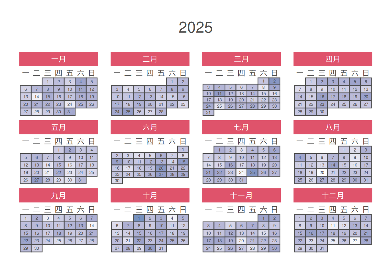

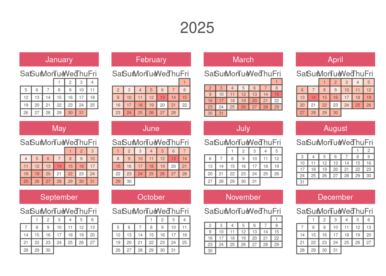
Chinese Calendar

2. English Calendar

# English Calendar
p <- calendR(
    year = 2025,
    month = NULL,
    from = NULL,
    to = NULL,
    start = "S",
    mbg.col = 2,
    # orientation = "portrait",
    months.col = "white",
    months.pos = 0.5,
    monthnames = c(
    "January",
    "February",
    "March",
    "April",
    "May",
    "June",
    "July",
    "August",
    "September",
    "October",
    "November",
    "December"
  ),
    weeknames = c("Sun", "Mon", "Tue", "Wed", "Thu", "Fri", "Sat"),
    special.days = data,
    special.col = "#00888888",
    gradient = TRUE,
    low.col = "#FFFFFF88",
    font.family = "sans",
    font.style = "plain",
    day.size = 2,
    # ncol = 2,
    lunar = FALSE,
    pdf = FALSE
)

p

English Calendar

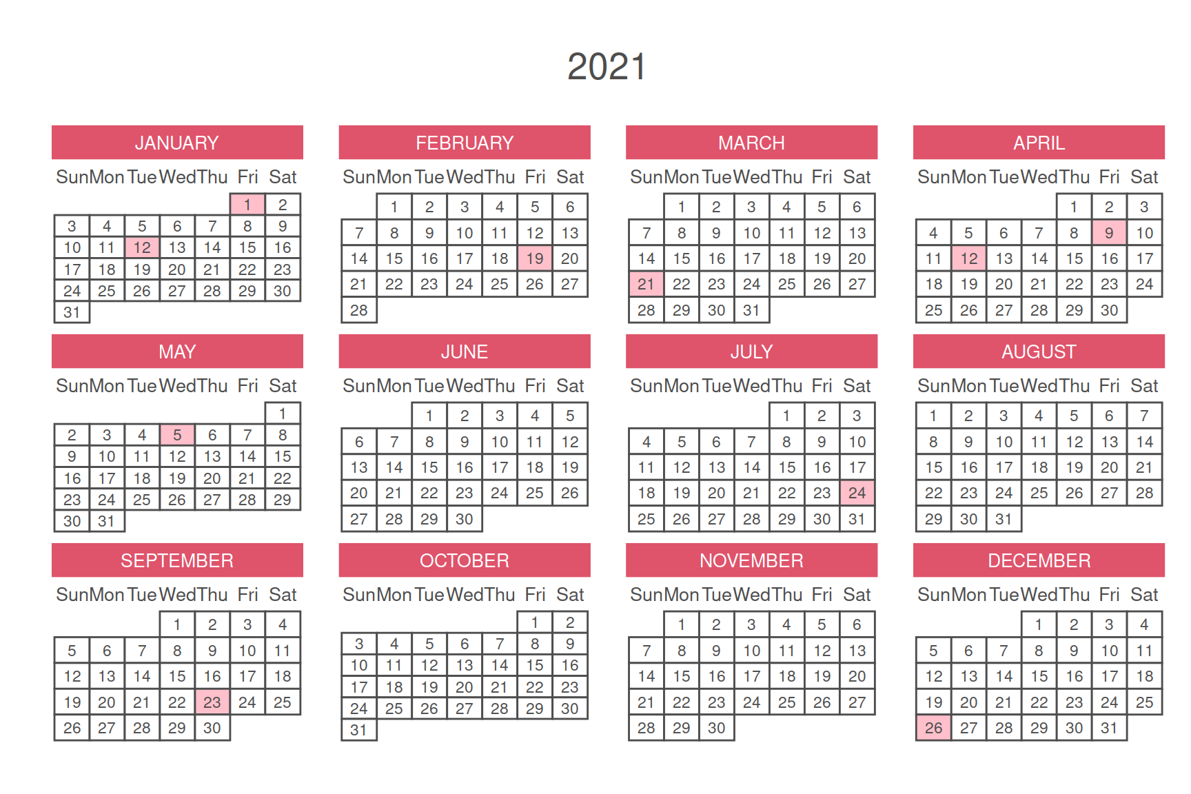
3. Calendar Period

# Calendar Period
data <- rnorm(30, 15, 10)
days <- rep(min(data) - 0.05, 365)
days[30:180] <- data

p <- calendR(
    year = 2025,
    month = NULL,
    from = NULL,
    to = NULL,
    start = "S",
    mbg.col = 2,
    # orientation = "portrait",
    months.col = "white",
    months.pos = 0.5,
    monthnames = c(
    "January",
    "February",
    "March",
    "April",
    "May",
    "June",
    "July",
    "August",
    "September",
    "October",
    "November",
    "December"
  ),
    weeknames = c("Sun", "Mon", "Tue", "Wed", "Thu", "Fri", "Sat"),
    special.days = days,
    special.col = "#FF000088",
    gradient = TRUE,
    low.col = "#FFFFFF88",
    font.family = "sans",
    font.style = "plain",
    day.size = 2,
    # ncol = 2,
    lunar = FALSE,
    pdf = FALSE
)

p

Calendar Period