# Install packages
if (!requireNamespace("data.table", quietly = TRUE)) {
  install.packages("data.table")
}
if (!requireNamespace("jsonlite", quietly = TRUE)) {
  install.packages("jsonlite")
}
if (!requireNamespace("plotROC", quietly = TRUE)) {
  install.packages("plotROC")
}
if (!requireNamespace("survivalROC", quietly = TRUE)) {
  install.packages("survivalROC")
}
if (!requireNamespace("ggplot2", quietly = TRUE)) {
  install.packages("ggplot2")
}
if (!requireNamespace("grid", quietly = TRUE)) {
  install.packages("grid")
}

# Load packages
library(data.table)
library(jsonlite)
library(plotROC)
library(survivalROC)
library(ggplot2)
library(grid)Time ROC
Note
Hiplot website
This page is the tutorial for source code version of the Hiplot Time ROC plugin. You can also use the Hiplot website to achieve no code ploting. For more information please see the following link:
Receiver Operating Characteristic (ROC) analysis with time records in survival analysis.
Setup
System Requirements: Cross-platform (Linux/MacOS/Windows)
Programming language: R
Dependent packages:
data.table;jsonlite;plotROC;survivalROC;ggplot2;grid
sessioninfo::session_info("attached")─ Session info ───────────────────────────────────────────────────────────────
setting value
version R version 4.6.0 (2026-04-24)
os Ubuntu 24.04.4 LTS
system x86_64, linux-gnu
ui X11
language (EN)
collate C.UTF-8
ctype C.UTF-8
tz UTC
date 2026-05-09
pandoc 3.1.3 @ /usr/bin/ (via rmarkdown)
quarto 1.9.37 @ /usr/local/bin/quarto
─ Packages ───────────────────────────────────────────────────────────────────
package * version date (UTC) lib source
data.table * 1.18.4 2026-05-06 [1] RSPM
ggplot2 * 4.0.3.9000 2026-05-04 [1] Github (tidyverse/ggplot2@6870419)
jsonlite * 2.0.0 2025-03-27 [1] RSPM
plotROC * 2.3.3 2025-08-25 [1] RSPM
survivalROC * 1.0.3.1 2022-12-05 [1] RSPM
[1] /home/runner/work/_temp/Library
[2] /opt/R/4.6.0/lib/R/site-library
[3] /opt/R/4.6.0/lib/R/library
* ── Packages attached to the search path.
──────────────────────────────────────────────────────────────────────────────Data Preparation
: (Numeric) survival data (i.e survive, risk). : (Numeric) time data.
# Load data
data1 <- data.table::fread(jsonlite::read_json("https://hiplot.cn/ui/basic/time-roc/data.json")$exampleData$textarea[[1]])
data1 <- as.data.frame(data1)
data2 <- data.table::fread(jsonlite::read_json("https://hiplot.cn/ui/basic/time-roc/data.json")$exampleData$textarea[[2]])
data2 <- as.data.frame(data2)

# convert data structure
surv_table <- data1
colnames(surv_table) <- c("surv", "cens", "risk")
mtime <- as.data.frame(data2)[, 1]
sroc <- lapply(mtime, function(t) {
  stroc <- survivalROC(
    Stime = surv_table$surv,
    status = surv_table$cens,
    marker = surv_table$risk,
    predict.time = t,
    method = "KM"
  )
  data.frame(
    TPF = stroc[["TP"]],
    FPF = stroc[["FP"]],
    cut = stroc[["cut.values"]],
    time = rep(
      stroc[["predict.time"]],
      length(stroc[["TP"]])
    ),
    AUC = rep(
      stroc$AUC,
      length(stroc$FP)
    )
  )
})
mroc <- do.call(rbind, sroc)
mroc$time <- factor(mroc$time)

# View data
head(data1)
surv cens risk
1 11.126027 0 0.19205450
2 9.794521 0 0.47734974
3 13.690411 0 0.04605343
4 10.068493 0 0.29717146
5 3.317808 0 0.18144610
6 12.312329 0 0.62681895head(data2) times
1 2
2 4
3 6
4 8
5 10Visualization
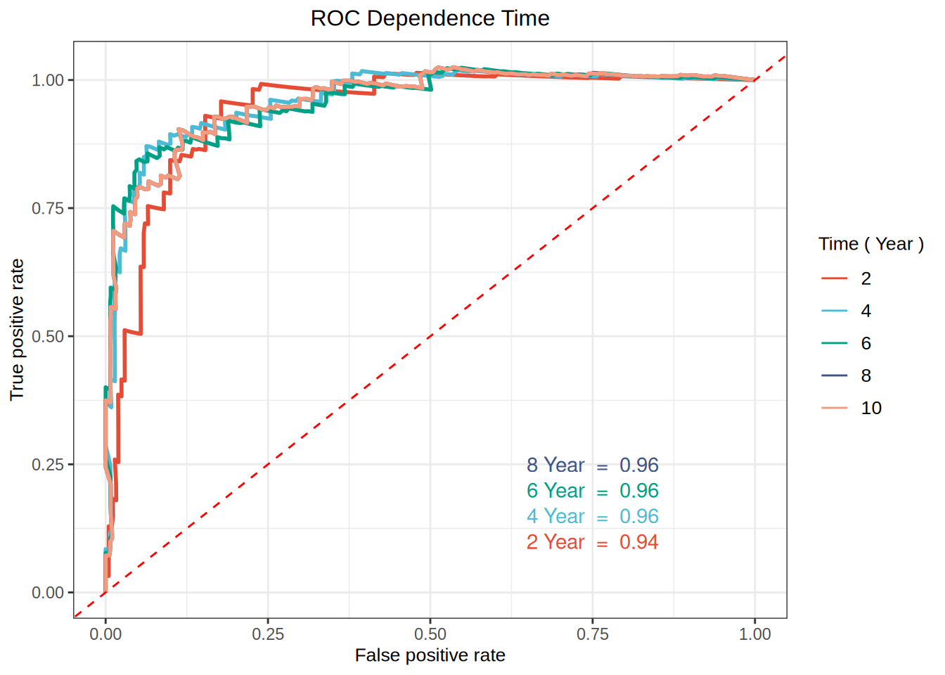
# Time ROC
col <- c("#E64B35FF","#4DBBD5FF","#00A087FF","#3C5488FF","#F39B7FFF")
p <- ggplot(mroc, aes(x = FPF, y = TPF, label = cut, color = time)) +
  plotROC::geom_roc(labels = FALSE, stat = "identity", n.cuts = 0) +
  geom_abline(slope = 1, intercept = 0, color = "red", linetype = 2) +
  labs(title = "ROC Dependence Time", x = "False positive rate",
       y = "True positive rate",
       color = paste("Time", "(", "Year", ")")) +
  theme_bw() +
  theme(text = element_text(family = "Arial"),
        plot.title = element_text(size = 12, hjust = 0.5),
        axis.title = element_text(size = 10),
        legend.position = "right",
        legend.direction = "vertical",
        legend.title = element_text(size = 10),
        legend.text = element_text(size = 10)) +
  scale_color_manual(values = col)

auc <- levels(factor(mroc$AUC))
for (i in 1:length(auc)) {
  p <- p + annotate("text",
    x = 0.75,
    y = 0.05 + 0.05 * i, ## 注释text的位置
    col = col[i],
    label = paste(
      paste(paste(mtime[i], "Year", sep = " "), " = "),
      round(as.numeric(auc[i]), 2)
    )
  )
}

p