Barplot Color Group

The color group barplot can be used to display data values in groups, and to label different colors in sequence.

Setup

• System Requirements: Cross-platform (Linux/MacOS/Windows)

• Programming language: R

• Dependent packages: data.table; jsonlite; ggplot2; stringr

# Install packages
if (!requireNamespace("data.table", quietly = TRUE)) {
  install.packages("data.table")
}
if (!requireNamespace("jsonlite", quietly = TRUE)) {
  install.packages("jsonlite")
}
if (!requireNamespace("ggplot2", quietly = TRUE)) {
  install.packages("ggplot2")
}
if (!requireNamespace("stringr", quietly = TRUE)) {
  install.packages("stringr")
}

# Load packages
library(data.table)
library(jsonlite)
library(ggplot2)
library(stringr)

Data Preparation

Data table (three columns):

Term | Entry name, such as GO/KEGG channel name

Count | The numerical size of the entry, such as the number of genes enriched in a pathway

Type | Category to which this channel belongs: such as BP/MF/CC/KEGG

# Load data
data <- data.table::fread(jsonlite::read_json("https://hiplot.cn/ui/basic/barplot-color-group/data.json")$exampleData$textarea[[1]])
data <- as.data.frame(data)

# convert data structure
colnames(data) <- c("term", "count", "type")
data[,"term"] <- str_to_sentence(str_remove(data[,"term"], pattern = "\\w+:\\d+\\W"))
data[,"term"] <- factor(data[,"term"], 
                        levels =  data[,"term"][length(data[,"term"]):1])
data[,"type"] <- factor(data[,"type"], 
                        levels = data[!duplicated(data[,"type"]), "type"])

# View data
data

                                                  term count type
1                                      Immune response    20   BP
2                        Defense response to bacterium    11   BP
3                                      Cell chemotaxis     8   BP
4                                        Cell adhesion    17   BP
5                                Complement activation     8   BP
6                  Cytokine-mediated signaling pathway     8   MF
7                             Phagocytosis, engulfment     5   MF
8              Negative regulation of jak-stat cascade     5   MF
9                             Epoxygenase p450 pathway     4   MF
10                Chemokine-mediated signaling pathway     6   MF
11  Negative regulation of leukocyte apoptotic process     3   MF
12                   B cell receptor signaling pathway     5   MF
13          Cellular response to tumor necrosis factor     6   CC
14                   Positive regulation of chemotaxis     3   CC
15                 Positive regulation of angiogenesis     6   CC
16                        Collagen fibril organization     4   CC
17 Positive regulation of homotypic cell-cell adhesion    20 KEGG
18              Regulation of cell projection assembly    14 KEGG
19                 Prostate epithelial cord elongation    10 KEGG
20                         Bile acid catabolic process     8 KEGG
21                           Cellular response to drug     7 KEGG
22                 Glycosaminoglycan metabolic process     4 KEGG

Visualization

# Barplot Color Group
p <- ggplot(data = data, aes(x = term, y = count, fill = type)) +
  geom_bar(stat = "identity", width = 0.8) + 
  theme_bw() +
  xlab("Count") +
  ylab("Term") +
  guides(fill = guide_legend(title="Type")) +
  ggtitle("Barplot Color Group") + 
  coord_flip() +
  theme_classic() +
  scale_fill_manual(values = c("#E64B35FF","#4DBBD5FF","#00A087FF","#3C5488FF")) +
  theme(text = element_text(family = "Arial"),
        plot.title = element_text(size = 12,hjust = 0.5),
        axis.title = element_text(size = 12),
        axis.text = element_text(size = 10),
        axis.text.x = element_text(angle = 0, hjust = 0.5,vjust = 1),
        legend.position = "right",
        legend.direction = "vertical",
        legend.title = element_text(size = 10),
        legend.text = element_text(size = 10))

p

Figure 1: Barplot Color Group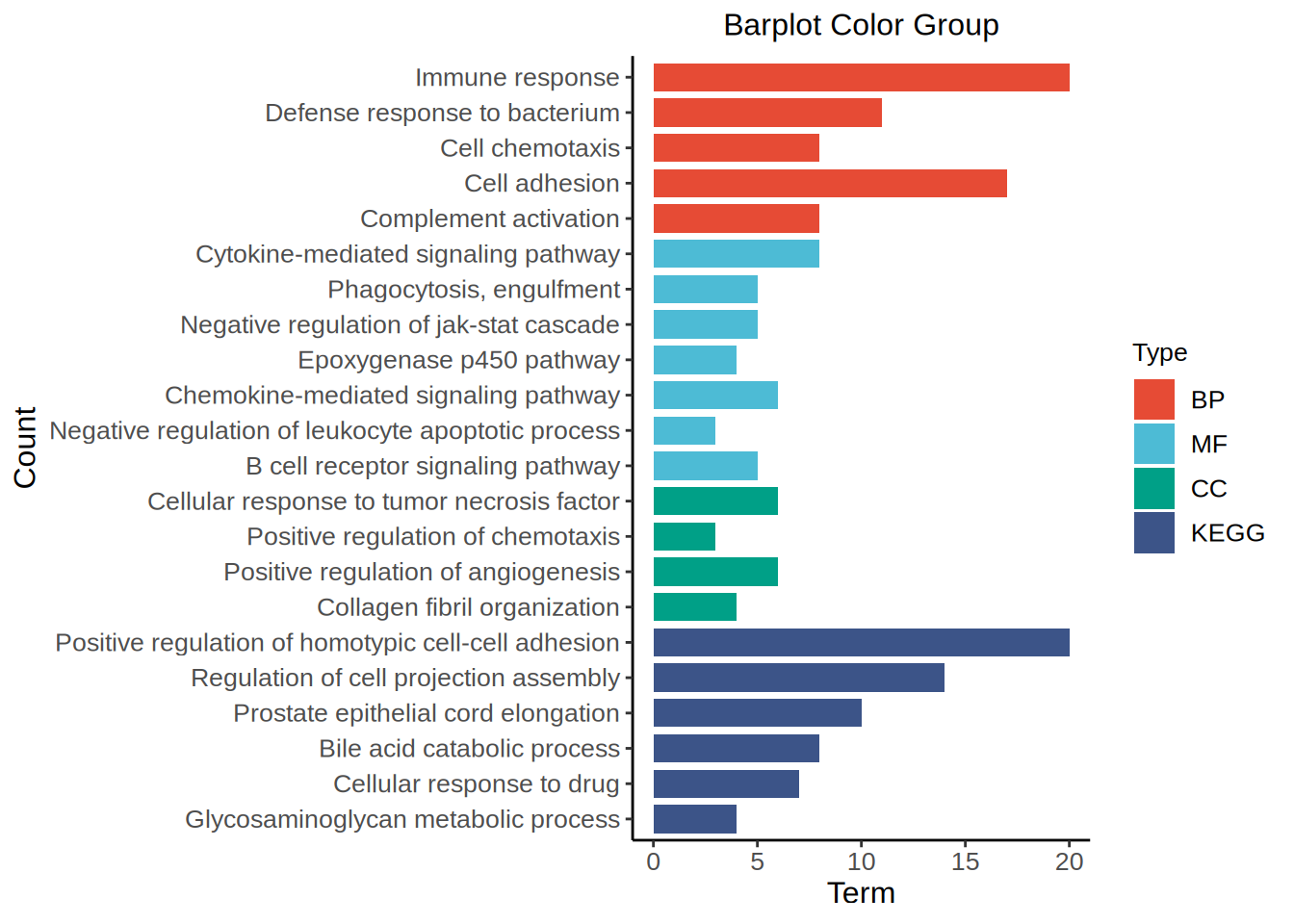

This plot visualizes the results of GO/KEGG pathway enrichment analysis.