# Installing necessary packages
if (!requireNamespace("forestploter", quietly = TRUE)) {
  install.packages("forestploter")
}

# Load packages
library(survival)
library(dplyr)
library(forestploter)
library(grid)Subgroup Forest Plot
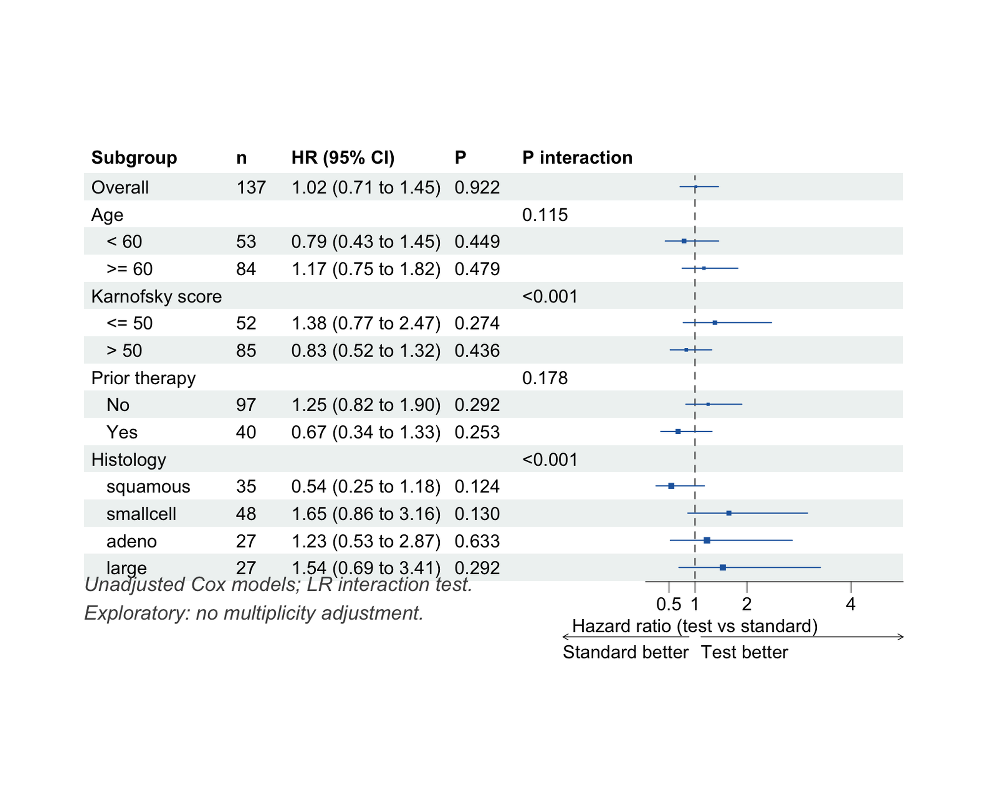
The subgroup forest plot summarizes a treatment effect (or any exposure effect) estimated within each level of baseline covariates — age groups, histology, disease severity — underneath the overall estimate. Each row shows the effect (e.g., a hazard ratio) with its 95% confidence interval as a square-and-whisker symbol; columns report the number of patients, the formatted estimate, and the within-subgroup p-value. A dedicated P interaction column tests whether the effect differs between subgroup levels [1].
Two statistical principles structure the plot. First, the interaction test — not the within-subgroup p-values — is the formal test of effect modification; a common reading error is to declare a subgroup effect from confidence intervals that merely cross the null line in one subgroup but not the other [2]. Second, subgroup findings are exploratory: they generate hypotheses for confirmation, and multiplicity across many subgroup variables should temper interpretation [1].
This tutorial builds a publication-grade subgroup forest plot with forestploter [3]:
- A basic subgroup forest of a survival treatment effect;
- The full publishable version — indented subgroup headers, interaction p-values, arrows and axis labels;
- A log-scale axis variant for strongly skewed hazard ratios.
Example
Setup
System Requirements: Cross-platform (Linux/MacOS/Windows)
Programming language: R
Dependent packages:
survival;dplyr;forestploter;grid
sessioninfo::session_info("attached")─ Session info ───────────────────────────────────────────────────────────────
setting value
version R version 4.6.2 (2026-10-29)
os Ubuntu 24.04.5 LTS
system x86_64, linux-gnu
ui X11
language (EN)
collate C.UTF-8
ctype C.UTF-8
tz UTC
date 2026-10-30
pandoc 3.1.3 @ /usr/bin/ (via rmarkdown)
quarto 1.10.19 @ /usr/local/bin/quarto
─ Packages ───────────────────────────────────────────────────────────────────
! package * version date (UTC) lib source
P dplyr * 1.2.1 2026-04-03 [?] RSPM
forestploter * 1.2.0 2026-09-30 [1] RSPM
P survival * 3.8-6 2026-01-16 [?] RSPM
[1] /home/runner/.cache/R/renv/library/Bizard-5140bdc6/linux-ubuntu-noble/R-4.6/x86_64-pc-linux-gnu
[2] /home/runner/work/_temp/Library
[3] /opt/R/4.6.2/lib/R/library
* ── Packages attached to the search path.
P ── Loaded and on-disk path mismatch.
──────────────────────────────────────────────────────────────────────────────Data Preparation
We use the built-in veteran data from the survival package [4]: a randomized trial of 137 lung-cancer patients comparing a standard versus a test chemotherapy (trt), with follow-up time, survival status and five baseline covariates. We dichotomize age (≥/< 60 years) and Karnofsky performance score (≤/> 50), keep prior therapy as a binary factor, and treat histology as a four-level factor. For each subgroup level we fit a Cox model of the treatment effect; for each subgroup variable we test the treatment × subgroup interaction by comparing models with and without the interaction term (likelihood-ratio test).
data(veteran, package = "survival")

vet <- veteran |>
  mutate(
    Age       = factor(ifelse(age >= 60, ">= 60", "< 60"), levels = c("< 60", ">= 60")),
    Karnofsky = factor(ifelse(karno <= 50, "<= 50", "> 50"), levels = c("<= 50", "> 50")),
    PriorTx   = factor(ifelse(prior == 0, "No", "Yes"), levels = c("No", "Yes")),
    Histology = relevel(factor(celltype), ref = "squamous")
  )

# Hazard ratio of the test vs standard arm within a subset of patients
sub_haz <- function(df) {
  fit <- coxph(Surv(time, status) ~ trt, data = df)
  s <- summary(fit)
  c(est = unname(s$coefficients["trt", "exp(coef)"]),
    lo  = unname(s$conf.int["trt", "lower .95"]),
    hi  = unname(s$conf.int["trt", "upper .95"]),
    n   = nrow(df),
    p   = unname(s$coefficients["trt", "Pr(>|z|)"]))
}

# Interaction p-value per subgroup variable: likelihood-ratio test of
# Cox(Surv ~ trt) vs Cox(Surv ~ trt * subgroup)
int_p <- function(var) {
  a <- anova(coxph(Surv(time, status) ~ trt, data = vet),
             coxph(as.formula(paste("Surv(time, status) ~ trt *", var)), data = vet))
  unname(a[2, "Pr(>|Chi|)"])
}

subgroups <- data.frame(
  label  = c("Age", "Karnofsky score", "Prior therapy", "Histology"),
  column = c("Age", "Karnofsky", "PriorTx", "Histology"),
  stringsAsFactors = FALSE
)
Visualization
1. Basic Subgroup Forest
Rows with NA estimates render as plain header rows, so we assemble the table with the overall row first, then each subgroup variable followed by its indented levels.
rows <- list(); hdr_p <- c()
add_row <- function(name, est = NA_real_, lo = NA_real_, hi = NA_real_,
                    n = NA_real_, p = NA_real_) {
  rows[[length(rows) + 1]] <<- data.frame(Subgroup = name, est = est, lo = lo, hi = hi,
                                          n = n, p = p, stringsAsFactors = FALSE)
}

r <- sub_haz(vet); add_row("Overall", r[["est"]], r[["lo"]], r[["hi"]], r[["n"]], r[["p"]])
for (i in seq_len(nrow(subgroups))) {
  v <- subgroups$column[i]
  add_row(subgroups$label[i])                       # header row: no estimate
  for (l in levels(vet[[v]])) {
    rr <- sub_haz(vet[vet[[v]] == l, ])
    add_row(paste0("   ", l), rr[["est"]], rr[["lo"]], rr[["hi"]], rr[["n"]], rr[["p"]])
  }
  hdr_p <- c(hdr_p, int_p(v))
}
sg <- dplyr::bind_rows(rows)

# Interaction p-values sit on the variable header rows
hdr_idx <- which(is.na(sg$est) & seq_len(nrow(sg)) > 1)
sg$`P interaction` <- ""
sg$`P interaction`[hdr_idx] <- ifelse(hdr_p < 0.001, "<0.001", sprintf("%.3f", hdr_p))

sg$`HR (95% CI)` <- ifelse(is.na(sg$est), "",
                           sprintf("%.2f (%.2f to %.2f)", sg$est, sg$lo, sg$hi))
sg$P <- ifelse(is.na(sg$p), "", ifelse(sg$p < 0.001, "<0.001", sprintf("%.3f", sg$p)))
sg$n <- ifelse(is.na(sg$n), "", as.character(sg$n))
sg$se <- (log(sg$hi) - log(sg$lo)) / (2 * 1.96)   # box size ~ CI width
sg$`  ` <- paste(rep(" ", 24), collapse = " ")     # blank spacer column for the CI

p <- forest(sg[, c("Subgroup", "n", "HR (95% CI)", "P", "P interaction", "  ")],
            est = sg$est, lower = sg$lo, upper = sg$hi,
            sizes = sg$se,
            ci_column = 6,
            ref_line = 1,
            xlim = c(0.05, 5),
            ticks_at = c(0.5, 1, 2, 4))
p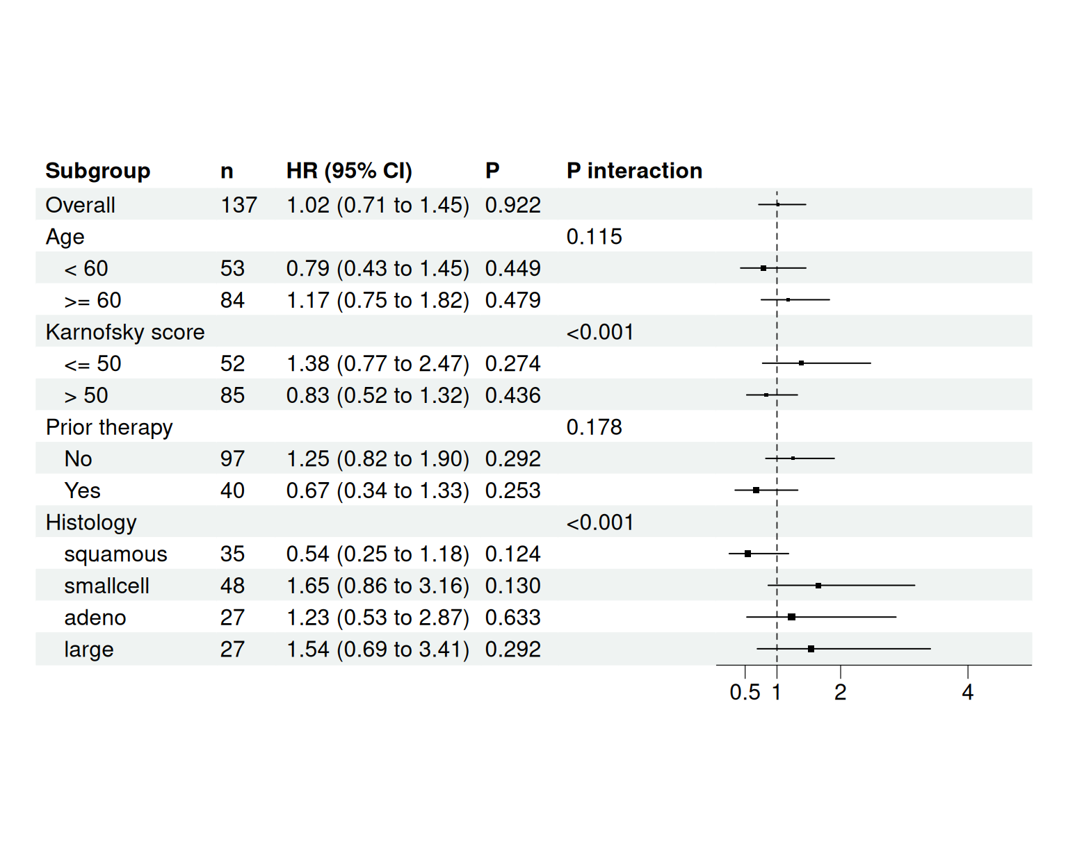
The overall hazard ratio is 1.02 (0.71 to 1.45): no evidence that the test chemotherapy changes mortality overall. The subgroup rows are where hypotheses live — but only the interaction column tells us whether any of the differences between subgroup levels are more than noise (see the next figure).
2. Publication Style: Interaction P, Arrows and Footnote
tm <- forest_theme(base_size = 11,
                   ci_pch = 15,
                   ci_col = "#2166AC",
                   ci_fill = "#2166AC",
                   refline_gp = gpar(col = "grey30", lty = 2),
                   footnote_gp = gpar(col = "grey30", fontface = "italic"))

p2 <- forest(sg[, c("Subgroup", "n", "HR (95% CI)", "P", "P interaction", "  ")],
             est = sg$est, lower = sg$lo, upper = sg$hi,
             sizes = sg$se,
             ci_column = 6,
             ref_line = 1,
             xlim = c(0.05, 5),
             ticks_at = c(0.5, 1, 2, 4),
             arrow_lab = c("Standard better", "Test better"),
             xlab = "Hazard ratio (test vs standard)",
             footnote = "Unadjusted Cox models; LR interaction test.\nExploratory: no multiplicity adjustment.",
             theme = tm)
p2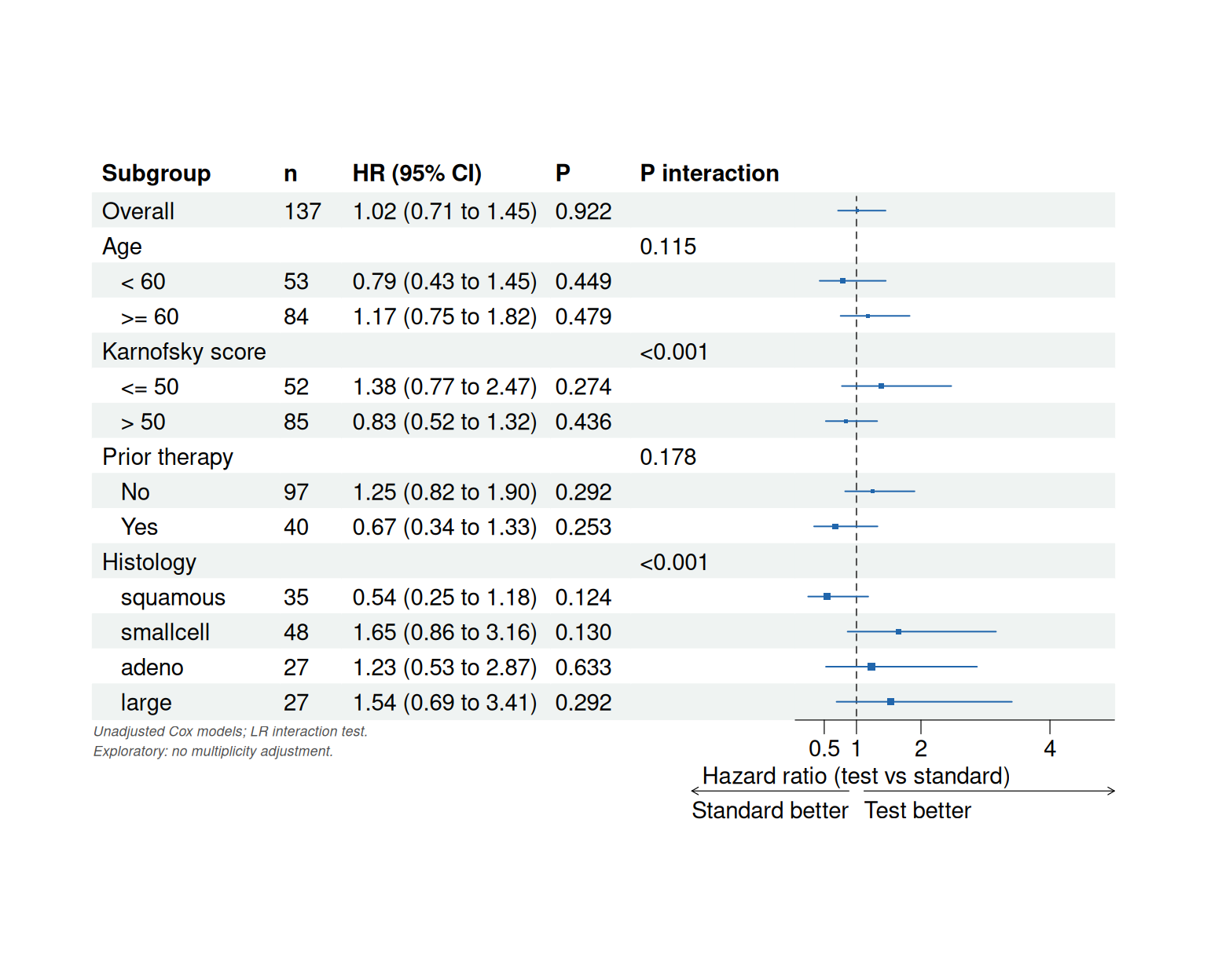
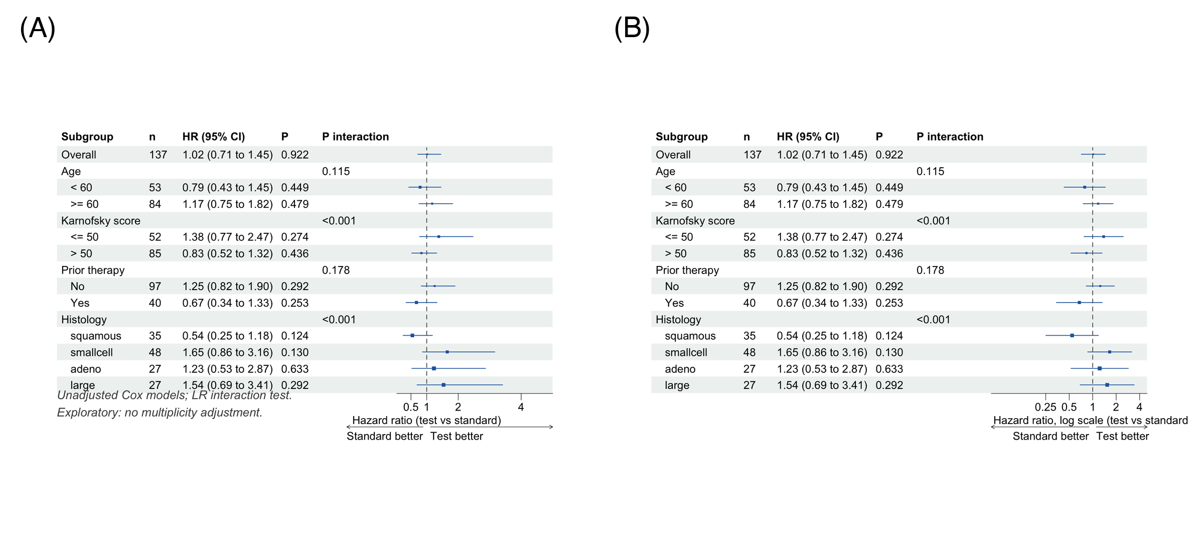
The strongly significant interactions for Karnofsky score (P < 0.001) and histology (P < 0.001) say the treatment effect differs across those subgroups. The point estimates suggest harm among patients with poor performance status (HR 1.38, 95% CI 0.77 to 2.47) and benefit in squamous histology (HR 0.54, 95% CI 0.25 to 1.18) — but both intervals include 1, which is exactly why the inference rests on the interaction test, not on the within-subgroup estimates. These are hypothesis-generating signals in a 137-patient trial, not confirmatory findings.
TipReading pitfalls
- Crossing confidence intervals are not an interaction test. “Significant in one subgroup, not in the other” is the null expectation whenever the true effect is identical in both — quote the P interaction instead [2].
- Multiplicity. Every added subgroup variable is another chance for a false positive; prespecify subgroups and report all of them, not only the significant ones.
- Interaction tests have low power. A non-significant P interaction does not prove homogeneous effects.
- Adjust or not, but say which. This example uses unadjusted within-subgroup models; many journals expect covariate-adjusted estimates, which change the numbers but not the workflow.
3. Log-Scale Axis for Skewed Intervals
p3 <- forest(sg[, c("Subgroup", "n", "HR (95% CI)", "P", "P interaction", "  ")],
             est = sg$est, lower = sg$lo, upper = sg$hi,
             sizes = sg$se,
             ci_column = 6,
             ref_line = 1,
             x_trans = "log",
             xlim = c(0.05, 5),
             ticks_at = c(0.25, 0.5, 1, 2, 4),
             arrow_lab = c("Standard better", "Test better"),
             xlab = "Hazard ratio, log scale (test vs standard)",
             theme = tm)
p3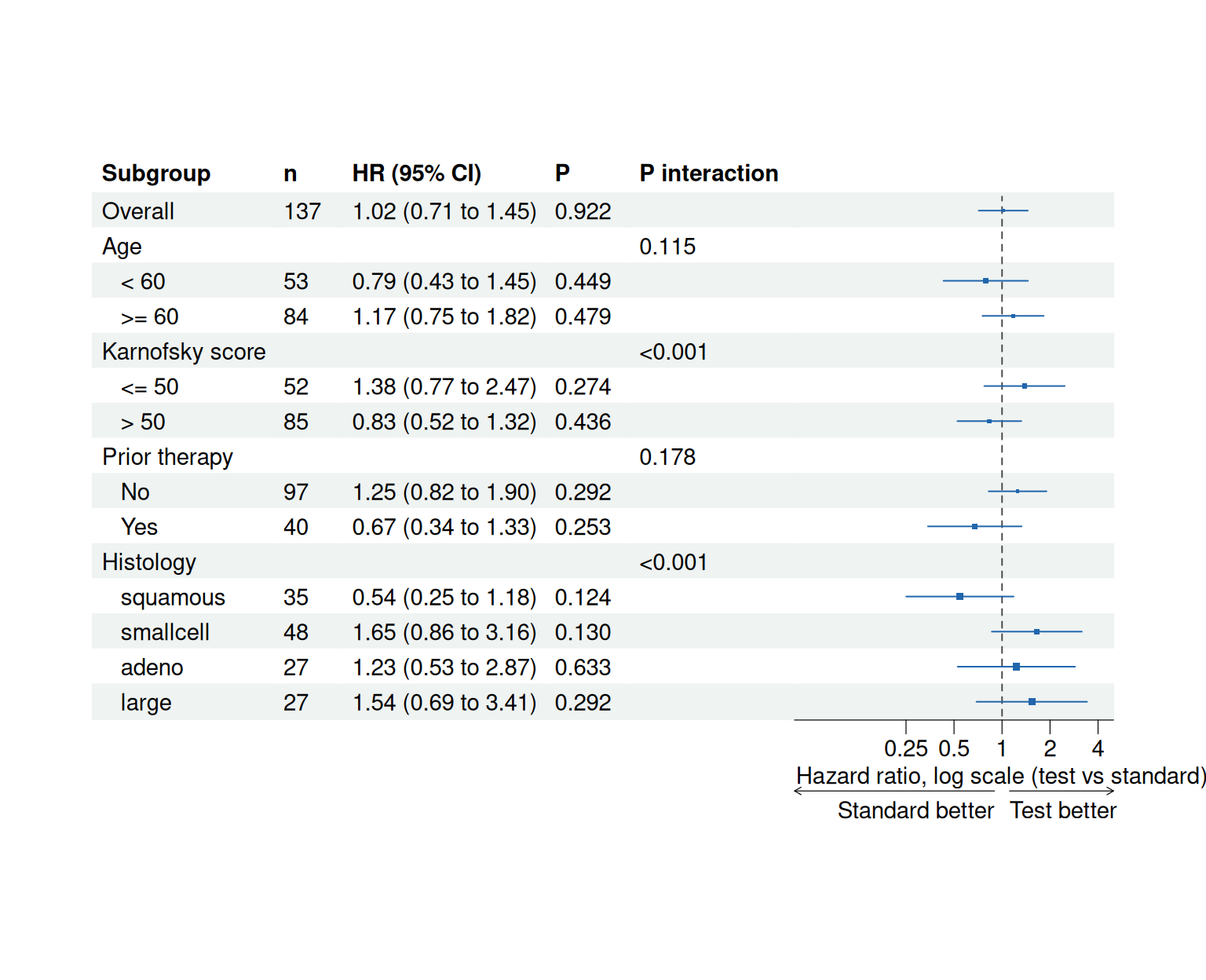
Hazard ratios are ratio measures, so a log axis is the geometrically honest display: a doubling (HR 2) and a halving (HR 0.5) get equal visual weight, and intervals appear symmetric around their estimate.
Application
Subgroup forest plots are a fixture of clinical trial reports (primary-paper Figure 1 in most NEJM/Lancet oncology trials), observational etiology papers, and biomarker-driven studies where the question is for whom the treatment works. The panel below mirrors that publication layout: (A) the standard subgroup forest and (B) the log-scale presentation used when intervals span an order of magnitude.
Reference
[1] Ballarini NM, Rosenkranz GK, Jaki T, König F, Posch M. A critical review of graphics for subgroup analyses in clinical trials. Pharm Stat. 2020;19(2):100-120. doi:10.1002/pst.2012
[2] Wang R, Lagakos SW, Ware JH, Hunter DJ, Drazen JM. Statistics in medicine — reporting of subgroup analyses in clinical trials. N Engl J Med. 2007;357(21):2189-2194. doi:10.1056/NEJMsr077003
[3] Dayimu A. forestploter: create a flexible forest plot. R package version 1.1.3. 2025. doi:10.32614/CRAN.package.forestploter
[4] Kalbfleisch JD, Prentice RL. The Statistical Analysis of Failure Time Data. New York: Wiley; 1980. (Veterans Administration lung cancer trial data)