import matplotlib.pyplot as plt
import networkx as nx
import numpy as npNetwork Plot (Python)
The Python counterpart of Network Plot — a node-link diagram places genes, proteins, or cell types as nodes and their relationships (co-expression, physical binding, communication) as edges. In biomedical research, network plots expose module structure and hub genes in co-expression analyses [1], summarize protein-interaction evidence, and visualize ligand-receptor inference from single-cell data.
networkx builds the graph and computes layouts; matplotlib draws [2]. Two properties decide whether a network plot communicates or misleads: the layout (positions are an optimization result, not coordinates) and visual encoding (node degree, edge weight, and module membership must map to size, width, and color consistently).
This tutorial covers three workflows:
- A spring-layout network with degree-coded node size and color;
- Spring vs Kamada-Kawai layouts side by side;
- Module-colored nodes with co-expression-weighted edges, plus a hub-subnetwork application panel.
Example
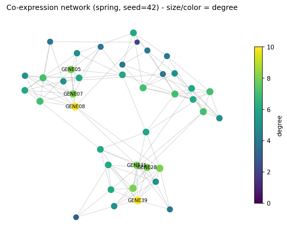
Setup
- System Requirements: Cross-platform (Linux/MacOS/Windows)
- Programming Language: Python
- Dependencies:
networkx,matplotlib,numpy
Data Preparation
We simulate a 40-gene co-expression module: three dense modules (14/13/13 genes) with strong within-module correlations, sparse inter-module bridges, and edge weights on a 0.3-0.95 scale. The same construction underlies real WGCNA-style exports [1].
rng = np.random.default_rng(7)
n_genes = 40
gene_names = [f"GENE{i:02d}" for i in range(1, n_genes + 1)]
modules = [(0, 14), (14, 27), (27, 40)]

G = nx.Graph()
G.add_nodes_from(gene_names)
for lo, hi in modules:                       # dense within-module edges
    for i in range(lo, hi):
        for j in range(i + 1, hi):
            if rng.random() < 0.45:
                G.add_edge(gene_names[i], gene_names[j],
                           weight=float(rng.uniform(0.55, 0.95)))
for i in range(n_genes):                     # sparse inter-module bridges
    for j in range(i + 1, n_genes):
        same = any(lo <= i < hi and lo <= j < hi for lo, hi in modules)
        if not same and rng.random() < 0.03:
            G.add_edge(gene_names[i], gene_names[j],
                       weight=float(rng.uniform(0.3, 0.5)))

degree = dict(G.degree())
# The layout is a randomized optimization: fix the seed or no two runs
# (and no two papers) look alike.
pos = nx.spring_layout(G, seed=42, k=0.6)
deg_arr = np.array([degree[g] for g in G.nodes()], dtype=float)
print(f"{G.number_of_nodes()} nodes, {G.number_of_edges()} edges, "
      f"max degree {int(deg_arr.max())}")
40 nodes, 119 edges, max degree 10Visualization
1. Degree-Coded Network
fig, ax = plt.subplots(figsize=(7, 5.6))
nx.draw_networkx_edges(G, pos, ax=ax, alpha=0.35, edge_color="grey",
                       width=0.8)
nc = nx.draw_networkx_nodes(G, pos, ax=ax, node_size=60 + 12 * deg_arr,
                            node_color=plt.cm.viridis(deg_arr / deg_arr.max()),
                            linewidths=0.4, edgecolors="white")
top = sorted(degree, key=degree.get, reverse=True)[:6]
nx.draw_networkx_labels(G, pos, labels={g: g for g in top},
                        font_size=8, ax=ax)
ax.set_title("Co-expression network (spring, seed=42) - size/color = degree")
ax.axis("off")
sm = plt.cm.ScalarMappable(cmap="viridis",
                           norm=plt.Normalize(0, deg_arr.max()))
fig.colorbar(sm, ax=ax, shrink=0.7, label="degree")
fig.tight_layout()
plt.show()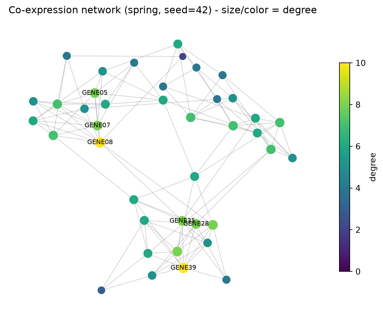
2. Layout Comparison: spring vs Kamada-Kawai
The spring layout is stochastic (hence the seed); Kamada-Kawai is deterministic and optimizes graph-theoretic distances. Same graph, different reading — show the layout you used.
pos_kk = nx.kamada_kawai_layout(G)
fig, axes = plt.subplots(1, 2, figsize=(11, 5))
for ax, (name, p) in zip(axes, [("spring_layout(seed=42)", pos),
                                ("kamada_kawai_layout", pos_kk)]):
    nx.draw_networkx_edges(G, p, ax=ax, alpha=0.3, edge_color="grey",
                           width=0.7)
    nx.draw_networkx_nodes(G, p, ax=ax, node_size=50 + 10 * deg_arr,
                           node_color="#4C72B0", linewidths=0.4,
                           edgecolors="white")
    ax.set_title(name); ax.axis("off")
fig.suptitle("Layout choice changes the reading", y=0.98)
fig.tight_layout()
plt.show()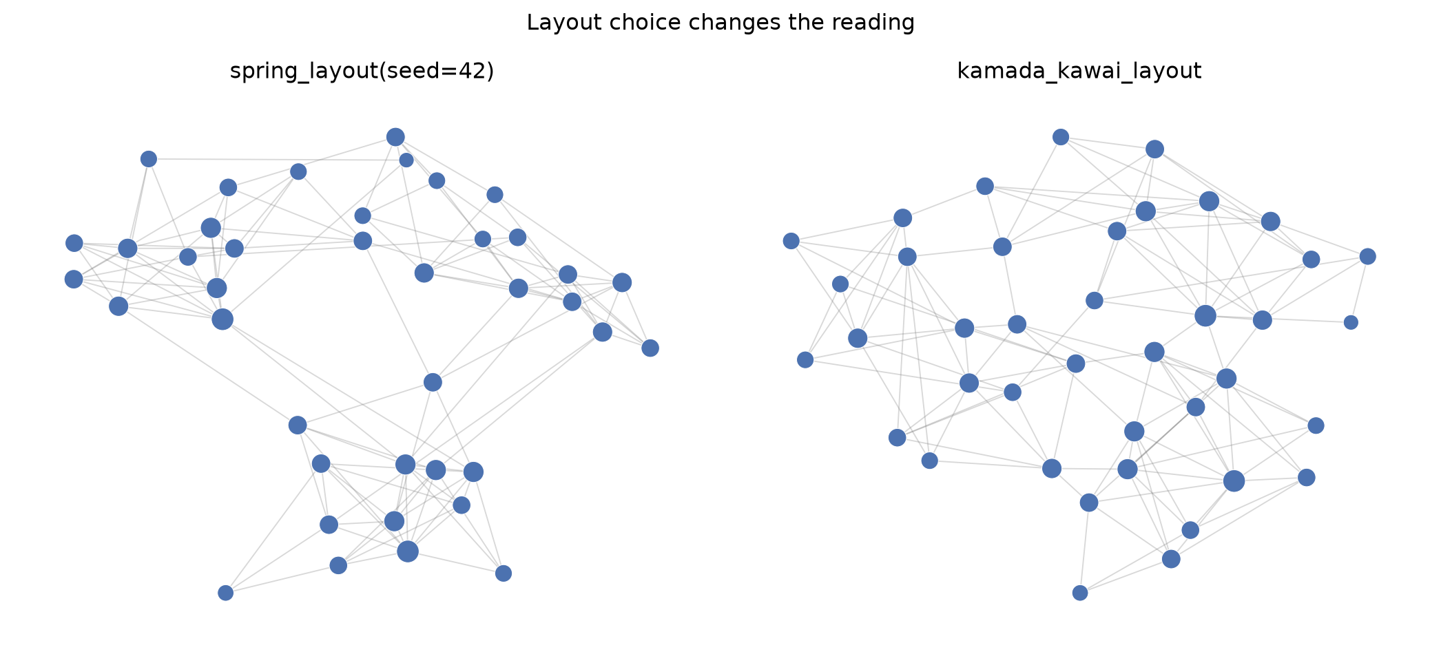
3. Module Colors and Weighted Edges
module_of = {}
for m, (lo, hi) in enumerate(modules):
    for i in range(lo, hi):
        module_of[gene_names[i]] = f"M{m + 1}"
mod_colors = {"M1": "#B2182B", "M2": "#2166AC", "M3": "#1B7837"}

fig, ax = plt.subplots(figsize=(7.4, 5.6))
edges, weights = zip(*[((u, v), d["weight"])
                       for u, v, d in G.edges(data=True)])
nx.draw_networkx_edges(G, pos, ax=ax, edgelist=edges,
                       width=[1 + 3.5 * w for w in weights],
                       edge_color=weights, edge_cmap=plt.cm.Greys,
                       edge_vmin=0.2, edge_vmax=1.0, alpha=0.75)
nx.draw_networkx_nodes(G, pos, ax=ax,
                       node_size=[60 + 12 * degree[g] for g in G.nodes()],
                       node_color=[mod_colors[module_of[g]] for g in G.nodes()],
                       linewidths=0.4, edgecolors="white")
nx.draw_networkx_labels(G, pos, labels={g: g for g in top},
                        font_size=8, ax=ax)
handles = [plt.Line2D([], [], marker="o", ls="", color=c, label=m)
           for m, c in mod_colors.items()]
ax.legend(handles=handles, loc="upper right", fontsize=9, title="module")
ax.set_title("Module-colored nodes; edge width/color = co-expression weight")
ax.axis("off")
fig.tight_layout()
plt.show()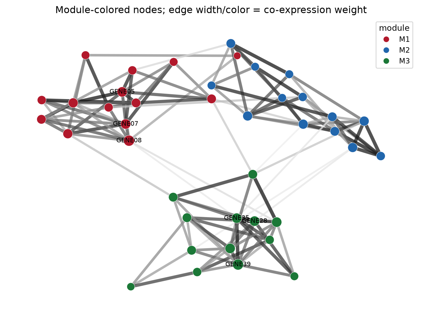
TipPractice tips
- Always seed
spring_layout(seed=) — an unseeded layout is not reproducible and reviewers cannot verify your figure. - Node degree in a thresholded network is a function of your cutoff; report the cutoff and prefer hub lists from the full weighted matrix.
- Do not encode two unrelated quantities in one channel (e.g., size = degree AND color = degree is redundant but fine; size = degree AND color = p-value invites misreading).
- Label only hub/annotated nodes — labelling all 40 nodes produces an unreadable wall of text.
- For interactive exploration, export the same graph with
nx.write_graphmland open it in Cytoscape [2].
Application
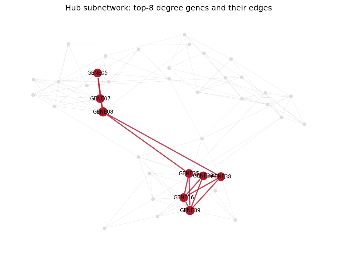
Hub analysis is the most common downstream readout: the panel below isolates the top-8 degree genes and the edges among them, turning a 40-node hairball into a testable hypothesis — hubs from different modules bridged by weak ties are candidates for experimental validation.
Reference
[1] Langfelder P, Horvath S. WGCNA: an R package for weighted correlation network analysis. BMC Bioinformatics. 2008;9:559. doi:10.1186/1471-2105-9-559
[2] Hagberg A, Schult D, Swart P. Exploring network structure, dynamics, and function using NetworkX. Proc 7th Python Sci Conf. 2008:11-15.