# Installing necessary packages
if (!requireNamespace("tidyverse", quietly = TRUE)) {
  install.packages("tidyverse")
}
if (!requireNamespace("scRNAtoolVis", quietly = TRUE)) {
  remotes::install_github("junjunlab/scRNAtoolVis")
}

# Load packages
library(tidyverse)
library(scRNAtoolVis)Bubble Heatmap
A bubble heatmap keeps the grid of a heatmap but replaces each colored cell with a bubble that can encode two variables at once: the bubble’s size carries one value (e.g. the fraction of cells expressing a gene) and its color carries another (e.g. the effect size or the significance). The result is the reference layout of single-cell marker dot plots and of pathway-enrichment matrices, where one glance reveals both how widespread and how strong each association is. This tutorial reproduces the chart type covered by the 顶刊图社 series (issue 013); see the Reference section below.
Example
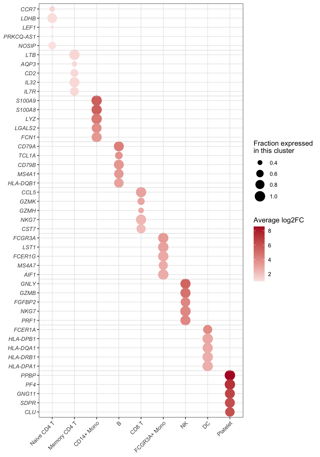
This bubble heatmap summarises the marker genes of the PBMC dataset: the top-5 markers of each of the nine cell clusters (45 marker rows — 44 unique genes, since NKG7 marks both CD8 T and NK cells — grouped into blocks of five by the faint separators) are plotted against the clusters. Bubble size is the fraction of cells of that cluster that express the gene (pct.1), and colour is the average log2 fold change of the gene against all remaining cells — the strongest marker of each cluster glows dark red in its own column, forming the diagonal.
Setup
System Requirements: Cross-platform (Linux/MacOS/Windows)
Programming Language: R
Dependencies:
tidyverse;scRNAtoolVis
Data Preparation
The example uses pbmc.markers, the PBMC single-cell marker table shipped with scRNAtoolVis (9 clusters, 5,921 marker statistics). Each row reports one gene in one cluster with the fraction of expressing cells (pct.1), the average log2 fold change (avg_log2FC) and the adjusted P value (p_val_adj). The top-5 markers per cluster give the figure its blocks.
data("pbmc.markers")

marker_top <- pbmc.markers |>
  group_by(cluster) |>
  slice_max(avg_log2FC, n = 5) |>
  ungroup() |>
  arrange(cluster, desc(avg_log2FC)) |>
  mutate(cluster = factor(cluster),
         row = row_number())

head(marker_top, 3)
# A tibble: 3 × 8
p_val avg_log2FC pct.1 pct.2 p_val_adj cluster gene row
<dbl> <dbl> <dbl> <dbl> <dbl> <fct> <chr> <int>
1 1.61e- 82 1.33 0.436 0.11 2.20e- 78 Naive CD4 T CCR7 1
2 1.96e-107 1.05 0.901 0.594 2.69e-103 Naive CD4 T LDHB 2
3 3.32e- 49 1.05 0.336 0.104 4.56e- 45 Naive CD4 T LEF1 3Note: In your own analysis the input is one row per row-column pair with the two values you want to encode — marker statistics from Seurat::FindAllMarkers(), a pathway enrichment table (gene count + P value), or any long-format matrix.
Visualization
1. Basic Plot
The basic figure maps pct.1 to bubble size and avg_log2FC to a diverging colour scale; genes are ordered block by block, so every cluster’s markers sit together.
ggplot(marker_top, aes(x = cluster, y = row)) +
  geom_point(aes(size = pct.1, colour = avg_log2FC)) +
  scale_colour_gradient2(low = "#2166ac", mid = "white", high = "#b2182b", midpoint = 0) +
  scale_size_continuous(range = c(1, 7)) +
  scale_y_continuous(breaks = marker_top$row, labels = marker_top$gene,
                     trans = "reverse", expand = expansion(add = .6)) +
  labs(x = NULL, y = NULL, colour = "avg log2FC", size = "pct.1") +
  theme_bw(base_size = 11) +
  theme(axis.text.y = element_text(face = "italic"),
        axis.text.x = element_text(angle = 45, hjust = 1))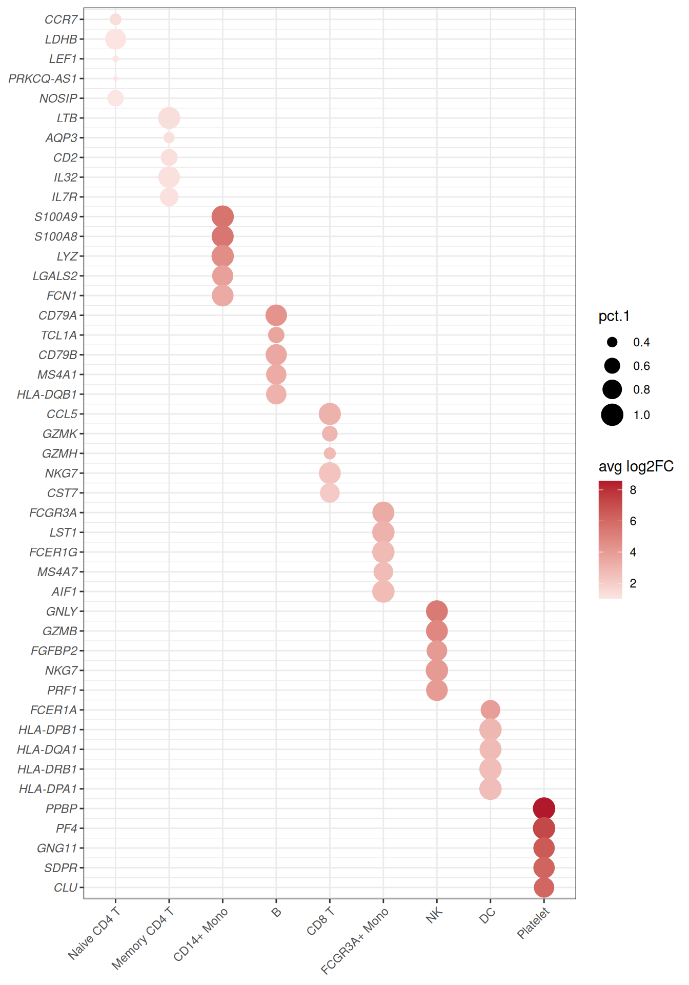
2. Refined Blocks and Legends
Faint separators between the gene blocks and descriptive legend titles turn the grid into the publication-ready dot plot; every bubble’s meaning is readable without the caption.
block_separators <- head(cumsum(table(marker_top$cluster)), -1) + 0.5

ggplot(marker_top, aes(x = cluster, y = row)) +
  geom_point(aes(size = pct.1, colour = avg_log2FC)) +
  geom_hline(yintercept = block_separators, colour = "grey85", linewidth = .3) +
  scale_colour_gradient2(low = "#2166ac", mid = "white", high = "#b2182b", midpoint = 0,
                         name = "Average log2FC") +
  scale_size_continuous(range = c(1, 7), name = "Fraction expressed\nin this cluster") +
  scale_y_continuous(breaks = marker_top$row, labels = marker_top$gene,
                     trans = "reverse", expand = expansion(add = .6)) +
  labs(x = NULL, y = NULL) +
  theme_bw(base_size = 11) +
  theme(panel.grid.minor = element_blank(),
        axis.text.y = element_text(face = "italic"),
        axis.text.x = element_text(angle = 45, hjust = 1))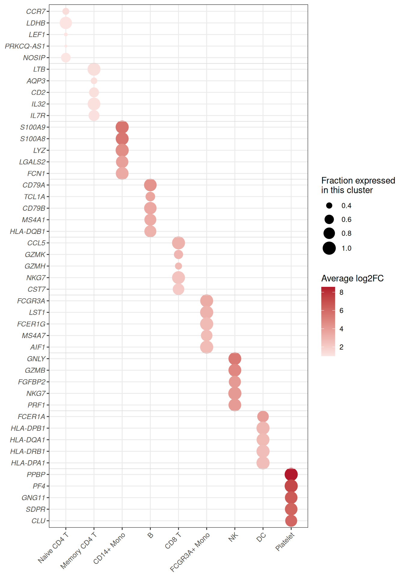
Tip
Key Parameters:
-
size = pct.1/colour = avg_log2FC: swap in any two numeric columns — the layout stays the same. -
range = c(1, 7): smallest and largest bubble size; keep the minimum above zero so absent values are visibly small, not invisible. -
midpoint = 0with a diverging scale: white marks the neutral value (here no fold change); usescale_colour_viridis_c()for strictly positive values (next figure).
3. Colour by Significance
The same grid can encode significance instead of effect size — the standard choice when the table comes from enrichment analysis, where -log10(P) spans orders of magnitude. Note the pmax() guard: p_val_adj is exactly 0 for the strongest markers, and -log10(0) would be infinite — clamping keeps those bubbles on the top of the scale instead of silently dropping them.
ggplot(marker_top, aes(x = cluster, y = row)) +
  geom_point(aes(size = pct.1, colour = -log10(pmax(p_val_adj, .Machine$double.xmin)))) +
  geom_hline(yintercept = block_separators, colour = "grey85", linewidth = .3) +
  scale_colour_viridis_c(option = "magma", direction = -1, name = expression(-log[10](P[adj]))) +
  scale_size_continuous(range = c(1, 7), name = "Fraction expressed\nin this cluster") +
  scale_y_continuous(breaks = marker_top$row, labels = marker_top$gene,
                     trans = "reverse", expand = expansion(add = .6)) +
  labs(x = NULL, y = NULL) +
  theme_bw(base_size = 11) +
  theme(panel.grid.minor = element_blank(),
        axis.text.y = element_text(face = "italic"),
        axis.text.x = element_text(angle = 45, hjust = 1))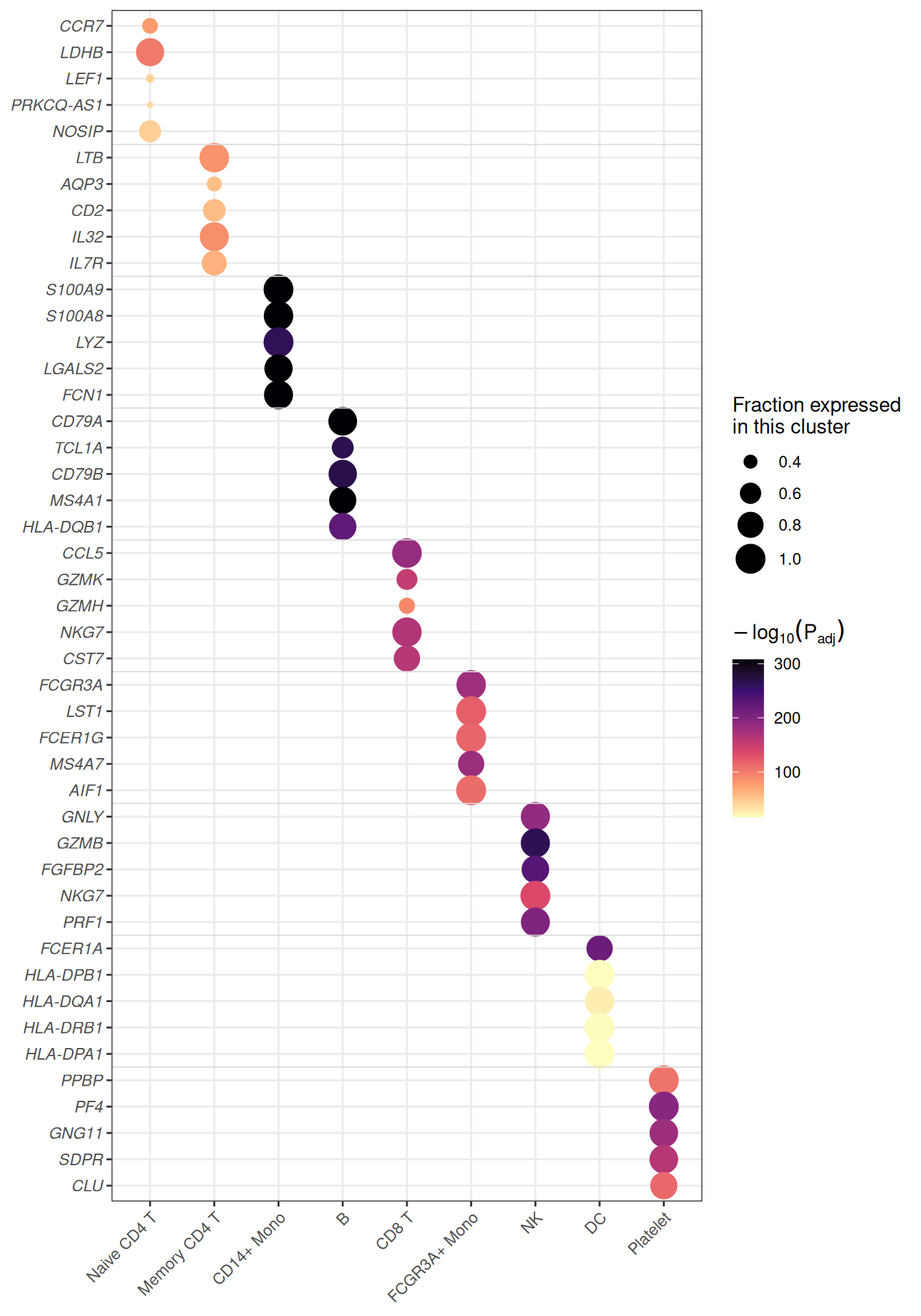
Applications
- Single-cell marker dot plots: the layout used across Seurat-style workflows to compare marker genes across clusters.
-
Enrichment matrices: pathways (rows) against clusters, conditions or time points (columns) with gene count as size and
-log10(P)as colour. - Cross-omics summaries: any two statistics per cell of a feature × sample grid — expression and significance, abundance and fold change, score and coverage.
- The bubbles are plain
geom_point()calls: no matrix reshaping is needed, only a long table with one row per grid cell.
Reference
[1] 顶刊图社 | 第013期:气泡热图. WeChat article. http://mp.weixin.qq.com/s?__biz=MzU5NjE2ODU0OQ==&mid=2247483869&idx=1&sn=f35b5747cffd6ee98d7fcf0148dc4752
[2] Zhang J. scRNAtoolVis: Making single-cell RNA-seq visualization easier and better. https://github.com/junjunlab/scRNAtoolVis (source of the pbmc.markers dataset).