# Installing necessary packages
if (!requireNamespace("ggplot2", quietly = TRUE)) {
  install.packages("ggplot2")
}
if (!requireNamespace("dplyr", quietly = TRUE)) {
  install.packages("dplyr")
}
if (!requireNamespace("tidyr", quietly = TRUE)) {
  install.packages("tidyr")
}
if (!requireNamespace("ggpubr", quietly = TRUE)) {
  install.packages("ggpubr")
}

# Load packages
library(ggplot2)
library(dplyr)
library(tidyr)
library(ggpubr)ChIP-seq Meta-Gene Profile with Significance
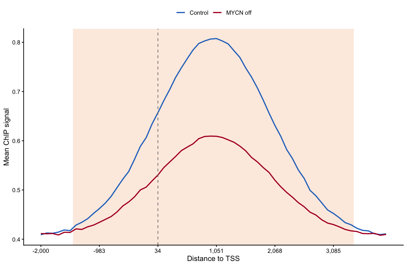
A quantitative (spike-in-corrected) ChIP-seq comparison is summarised by a meta-gene profile: signal averaged over all active genes across the TSS and gene body, with a Welch t test per bin marking where two conditions differ globally [1]. The companion travel-ratio (TR) boxplots condense the same comparison to one number per gene. This tutorial draws both from simulated bigWig-style matrices — the plotting half of the bigWigSummary workflow.
Example
Setup
System Requirements: Cross-platform (Linux/MacOS/Windows)
Programming Language: R
Dependent packages:
ggplot2;dplyr;tidyr;ggpubr
sessioninfo::session_info("attached")─ Session info ───────────────────────────────────────────────────────────────
setting value
version R version 4.6.2 (2026-10-29)
os Ubuntu 26.04.1 LTS
system x86_64, linux-gnu
ui X11
language (EN)
collate C.UTF-8
ctype C.UTF-8
tz UTC
date 2026-11-05
pandoc 3.7.0.2 @ /usr/bin/ (via rmarkdown)
quarto 1.11.9 @ /usr/local/bin/quarto
─ Packages ───────────────────────────────────────────────────────────────────
! package * version date (UTC) lib source
P dplyr * 1.2.1 2026-04-03 [?] RSPM
P ggplot2 * 4.0.3.9000 2026-11-03 [?] Github (tidyverse/ggplot2@b638d65)
P ggpubr * 1.0.0 2026-07-06 [?] RSPM
P tidyr * 1.3.2 2025-12-19 [?] RSPM
[1] /home/runner/.cache/R/renv/library/Bizard-5140bdc6/linux-ubuntu-resolute/R-4.6/x86_64-pc-linux-gnu
[2] /home/runner/work/_temp/Library
[3] /opt/R/4.6.2/lib/R/library
* ── Packages attached to the search path.
P ── Loaded and on-disk path mismatch.
──────────────────────────────────────────────────────────────────────────────Data Preparation
In practice you extract per-gene binned signal with the UCSC bigWigSummary utility (one row per gene, one column per bin, per condition) and read the tables into R. We simulate 1,000 active genes over 60 bins spanning −2 kb … +4 kb around the TSS, in a control and an MYCN-shutdown condition with a genome-wide loss of promoter signal.
set.seed(801)
n_gene <- 1000
n_bin <- 60
genes <- paste0("GENE", sprintf("%04d", 1:n_gene))

shape <- dnorm(seq(-3, 3, length.out = n_bin))          # promoter-peaked profile
ctrl <- t(sapply(1.6 ^ rnorm(n_gene, 0, 0.35), function(depth)     # genes as rows
  depth * (0.4 + shape) + rnorm(n_bin, sd = 0.05)))
knockdown <- t(sapply(1.6 ^ rnorm(n_gene, 0, 0.35), function(depth)
  depth * (0.4 + 0.5 * shape) + rnorm(n_bin, sd = 0.05)))

colnames(ctrl) <- paste0("ctrl_b", sprintf("%02d", 1:n_bin))
colnames(knockdown) <- paste0("kd_b", sprintf("%02d", 1:n_bin))

## travel ratio: promoter signal (first 10 bins) / total signal over the window
tr <- function(m) rowSums(m[, 1:10]) / rowSums(m)
tr_df <- data.frame(gene = rep(genes, times = 2),
                    Condition = rep(factor(c("Control", "MYCN off"),
                                           levels = c("Control", "MYCN off")),
                                    each = n_gene),
                    TR = c(tr(ctrl), tr(knockdown)))
head(tr_df, 3)
gene Condition TR
1 GENE0001 Control 0.1242675
2 GENE0002 Control 0.1276115
3 GENE0003 Control 0.1298037Visualization
1. Meta-Gene Profile with Per-Bin Significance
bin_pos <- seq(-2000, 4000, length.out = n_bin)
meta <- data.frame(
  bin = seq_len(n_bin),
  ctrl_mean = colMeans(ctrl),
  ctrl_se = apply(ctrl, 2, function(x) sd(x) / sqrt(n_gene)),
  kd_mean = colMeans(knockdown),
  kd_se = apply(knockdown, 2, function(x) sd(x) / sqrt(n_gene)),
  p = sapply(seq_len(n_bin), function(b)
    t.test(ctrl[, b], knockdown[, b], var.equal = FALSE)$p.value))

meta_df <- meta |>
  pivot_longer(cols = c(ctrl_mean, kd_mean), names_to = "condition", values_to = "mean") |>
  mutate(se = ifelse(condition == "ctrl_mean", meta$ctrl_se, meta$kd_se),
         condition = ifelse(condition == "ctrl_mean", "Control", "MYCN off"))
sig_band <- subset(meta, p < 0.05)

ggplot() +
  geom_rect(data = sig_band, inherit.aes = FALSE,
            aes(xmin = bin - 0.5, xmax = bin + 0.5, ymin = -Inf, ymax = Inf),
            fill = "#FDE7DA", alpha = 0.8) +
  geom_ribbon(data = meta_df, aes(bin, ymin = mean - se, ymax = mean + se, fill = condition),
              alpha = 0.25, colour = NA) +
  geom_line(data = meta_df, aes(bin, mean, colour = condition), linewidth = 0.9) +
  geom_vline(xintercept = which.min(abs(bin_pos)), linetype = "dashed", colour = "grey50") +
  annotate("text", x = which.min(abs(bin_pos)) + 1.5,
           y = max(meta_df$mean) * 1.02, label = "TSS", hjust = 0, size = 3) +
  scale_x_continuous(breaks = seq(1, n_bin, 10),
                     labels = scales::comma(bin_pos[seq(1, n_bin, 10)])) +
  scale_colour_manual(values = c(Control = "#2874C5", `MYCN off` = "#B2182B")) +
  scale_fill_manual(values = c(Control = "#2874C5", `MYCN off` = "#B2182B")) +
  labs(x = "Distance to TSS", y = "Mean ChIP signal",
       title = "Meta-gene profile, all active genes",
       subtitle = "Shaded bins: Welch p < 0.05", colour = NULL, fill = NULL) +
  theme_classic(base_size = 11) +
  theme(legend.position = "top", legend.key.size = unit(3, "mm"))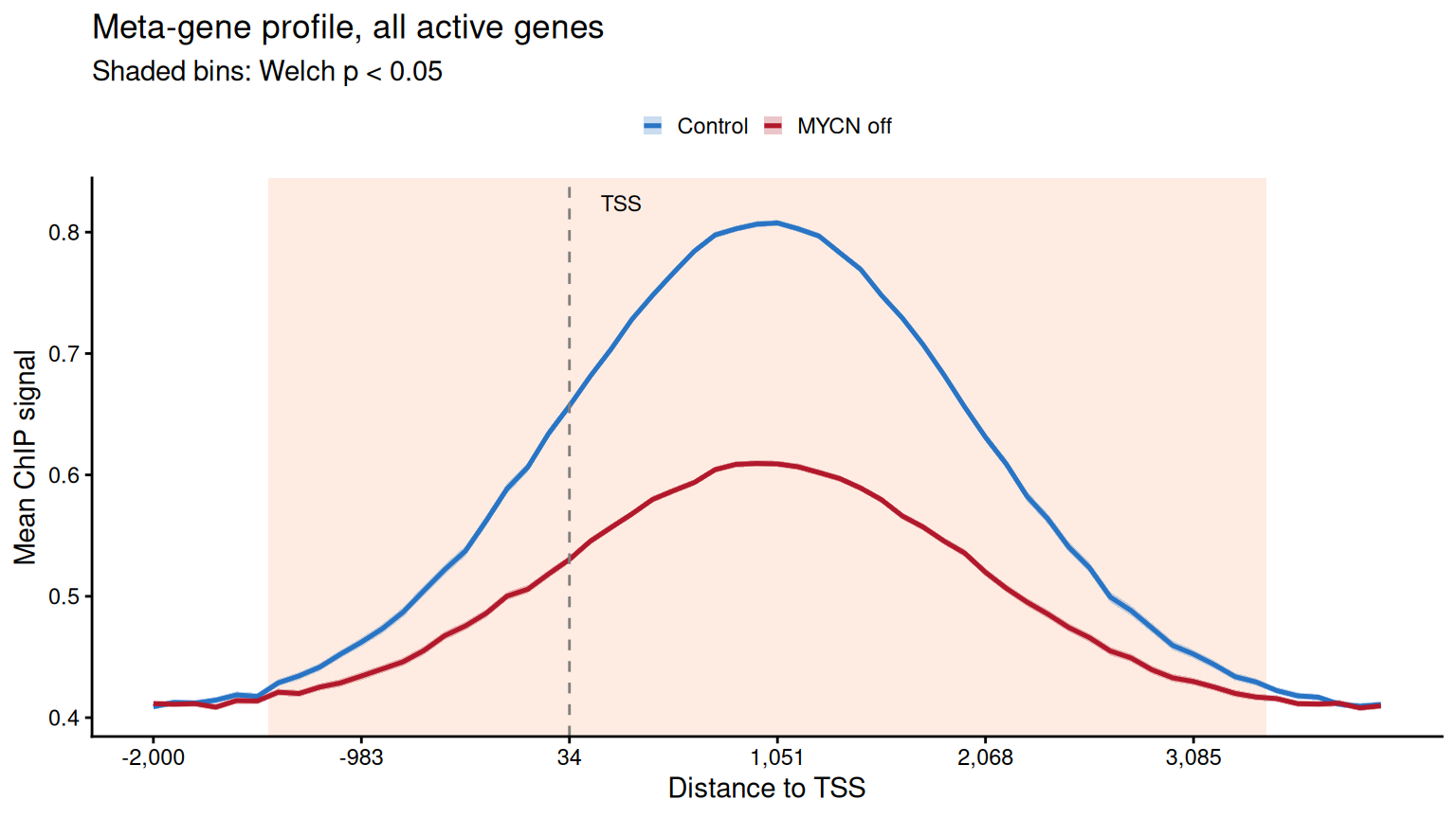
2. Travel-Ratio Distributions with Significance Stars
p_tr <- t.test(TR ~ Condition, data = tr_df, var.equal = FALSE)$p.value
star <- cut(p_tr, c(0, 1e-9, 1e-6, 1e-3, 1),
            labels = c("****", "***", "**", "*"))

ggplot(tr_df, aes(Condition, TR, fill = Condition)) +
  geom_boxplot(outlier.shape = NA, width = 0.55) +
  geom_jitter(width = 0.08, size = 0.4, alpha = 0.25, show.legend = FALSE) +
  scale_fill_manual(values = c(Control = "#BDD7E7", `MYCN off` = "#FCAE91")) +
  labs(y = "RNA Pol II travelling ratio", title = sprintf("Welch p %s",
       ifelse(p_tr < 0.001, "< 0.001", sprintf("= %.3f", p_tr)))) +
  theme_classic(base_size = 11) +
  theme(legend.position = "none")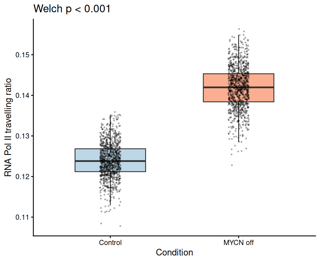
Tip
Practice tips
- The meta-gene test is only meaningful on normalised (spike-in-corrected) data — global uncorrected losses are exactly the artefact the reference paper guards against.
- A Welch (unequal-variance) t test per bin is the reference statistic; display the p band as a background ribbon rather than stars per bin, which becomes unreadable at 60 bins.
- The TR (travelling ratio, promoter / total) needs a fixed gene set — use “all active genes” consistently across conditions or the comparison is confounded.
Application
Meta-gene profiles with per-bin significance are the standard first figure for global ChIP-seq comparisons (transcription-factor shutdown, drug treatment). The same code accepts any two conditions’ binned matrices.
Reference
[1] Deregulated MYCN binds active chromatin and amplifies transcription in neuroblastoma. Nat Genet. 2018. https://www.nature.com/articles/s41588-018-0044-9 (reference figure context)
[2] Xiaofan Lu, et al. FigureYa: A Standardized Visualization Framework for Enhancing Biomedical Data Interpretation and Research Efficiency. iMetaMed. 2025. doi:10.1002/imm3.70005