# Installing necessary packages
if (!requireNamespace("ComplexHeatmap", quietly = TRUE)) {
  BiocManager::install("ComplexHeatmap")
}
if (!requireNamespace("ggplot2", quietly = TRUE)) {
  install.packages("ggplot2")
}
if (!requireNamespace("dplyr", quietly = TRUE)) {
  install.packages("dplyr")
}
if (!requireNamespace("tidyr", quietly = TRUE)) {
  install.packages("tidyr")
}
if (!requireNamespace("circlize", quietly = TRUE)) {
  install.packages("circlize")
}
if (!requireNamespace("ggpubr", quietly = TRUE)) {
  install.packages("ggpubr")
}

# Load packages
library(ComplexHeatmap)
library(ggplot2)
library(dplyr)
library(tidyr)
library(circlize)
library(ggpubr)Single-Cell Pathway Scores (GSVA)
After annotating single-cell subpopulations, the recurring question is how active a pathway is in each cell or cluster, and whether two clusters differ [1]. GSVA scores every cell for a gene set; the scores are then compared between clusters with a heatmap and a boxplot. This tutorial runs that workflow on a simulated cells × genes matrix — the plotting half of the reference pipeline (matrix → grouping → GSVA → figure).
Example

Setup
System Requirements: Cross-platform (Linux/MacOS/Windows)
Programming Language: R
Dependent packages:
ComplexHeatmap;ggplot2;dplyr;tidyr;circlize;ggpubr
sessioninfo::session_info("attached")─ Session info ───────────────────────────────────────────────────────────────
setting value
version R version 4.6.2 (2026-10-29)
os Ubuntu 26.04.1 LTS
system x86_64, linux-gnu
ui X11
language (EN)
collate C.UTF-8
ctype C.UTF-8
tz UTC
date 2026-11-05
pandoc 3.7.0.2 @ /usr/bin/ (via rmarkdown)
quarto 1.11.9 @ /usr/local/bin/quarto
─ Packages ───────────────────────────────────────────────────────────────────
! package * version date (UTC) lib source
P circlize * 0.4.18 2026-04-04 [?] RSPM
P ComplexHeatmap * 2.28.0 2026-04-28 [?] Bioconductor 3.23 (R 4.6.2)
P dplyr * 1.2.1 2026-04-03 [?] RSPM
P ggplot2 * 4.0.3.9000 2026-11-03 [?] Github (tidyverse/ggplot2@b638d65)
P ggpubr * 1.0.0 2026-07-06 [?] RSPM
P tidyr * 1.3.2 2025-12-19 [?] RSPM
[1] /home/runner/.cache/R/renv/library/Bizard-5140bdc6/linux-ubuntu-resolute/R-4.6/x86_64-pc-linux-gnu
[2] /home/runner/work/_temp/Library
[3] /opt/R/4.6.2/lib/R/library
* ── Packages attached to the search path.
P ── Loaded and on-disk path mismatch.
──────────────────────────────────────────────────────────────────────────────Data Preparation
We simulate log-normalised expression for 400 cells from two endothelial-like subpopulations (EC1, EC2) and six hallmark-like pathways planted with cluster-specific activity — the state right before GSVA in the reference workflow.
set.seed(1001)
n_cell <- 200                                     # per cluster
genes <- paste0("Gene", sprintf("%04d", 1:300))
cells <- c(paste0("EC1_", sprintf("%03d", 1:n_cell)),
           paste0("EC2_", sprintf("%03d", 1:n_cell)))
cluster <- factor(rep(c("EC1", "EC2"), each = n_cell), levels = c("EC1", "EC2"))

expr <- matrix(rnorm(300 * 2 * n_cell, sd = 0.5), nrow = 300,
               dimnames = list(genes, cells))
pathways <- list(
  "Angiogenesis"       = 1:40,    "EC activation"     = 41:80,
  "Hypoxia"            = 81:110,  "Leukocyte migration" = 111:150,
  "Coagulation"        = 151:180, "Antigen processing"  = 181:210
)
signal <- c(1.4, 1.0, 0.6, -0.3, 0, 0)             # EC1 > EC2 for the first three
for (k in seq_along(pathways)) {
  pg <- names(pathways)[k]
  expr[pathways[[pg]], cluster == "EC1"] <-
    expr[pathways[[pg]], cluster == "EC1"] + signal[k]
}
Visualization
1. Per-Cell Pathway Scores (GSVA Heatmap)
## Dependency-free per-cell set score (mean of set genes); the reference
## workflow uses GSVA::gsva() on the normalised matrix — same input, same layout
score_mat <- t(sapply(pathways, function(idx) colMeans(expr[idx, , drop = FALSE])))
score_z <- t(scale(t(score_mat)))

ha <- HeatmapAnnotation(Cluster = cluster,
                        col = list(Cluster = c(EC1 = "#B31E22", EC2 = "#529B40")),
                        show_legend = FALSE)
col_fun <- circlize::colorRamp2(c(-2, 0, 2), c("#2166AC", "white", "#B2182B"))
Heatmap(score_z, name = "Score (z)",
        top_annotation = ha, col = col_fun,
        cluster_columns = FALSE,
        column_split = cluster, column_gap = unit(1.5, "mm"),
        row_names_gp = grid::gpar(fontsize = 9),
        show_column_names = FALSE, border = TRUE)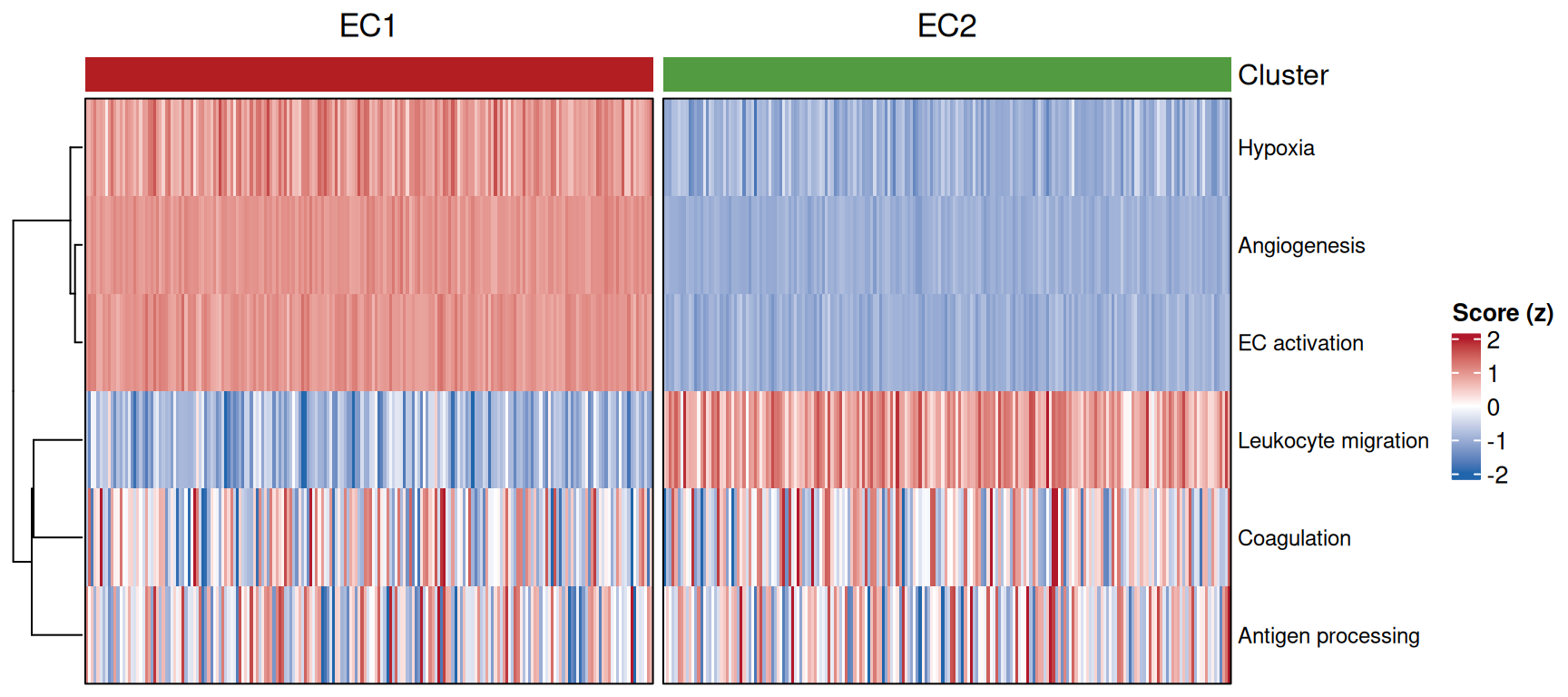
2. Comparing a Pathway Between Clusters
box_df <- data.frame(cluster = cluster,
                     score = score_mat["Angiogenesis", ])
p_kw <- wilcox.test(score ~ cluster, data = box_df)$p.value

ggplot(box_df, aes(cluster, score, fill = cluster)) +
  geom_boxplot(outlier.shape = NA, width = 0.55) +
  geom_jitter(width = 0.15, size = 0.5, alpha = 0.4, show.legend = FALSE) +
  scale_fill_manual(values = c(EC1 = "#B31E22", EC2 = "#529B40")) +
  labs(title = sprintf("Angiogenesis (Wilcoxon %s)",
       ifelse(p_kw < 0.001, "p < 0.001", sprintf("p = %.3f", p_kw))),
       x = NULL, y = "Pathway score", fill = NULL) +
  theme_classic(base_size = 11) +
  theme(legend.position = "none")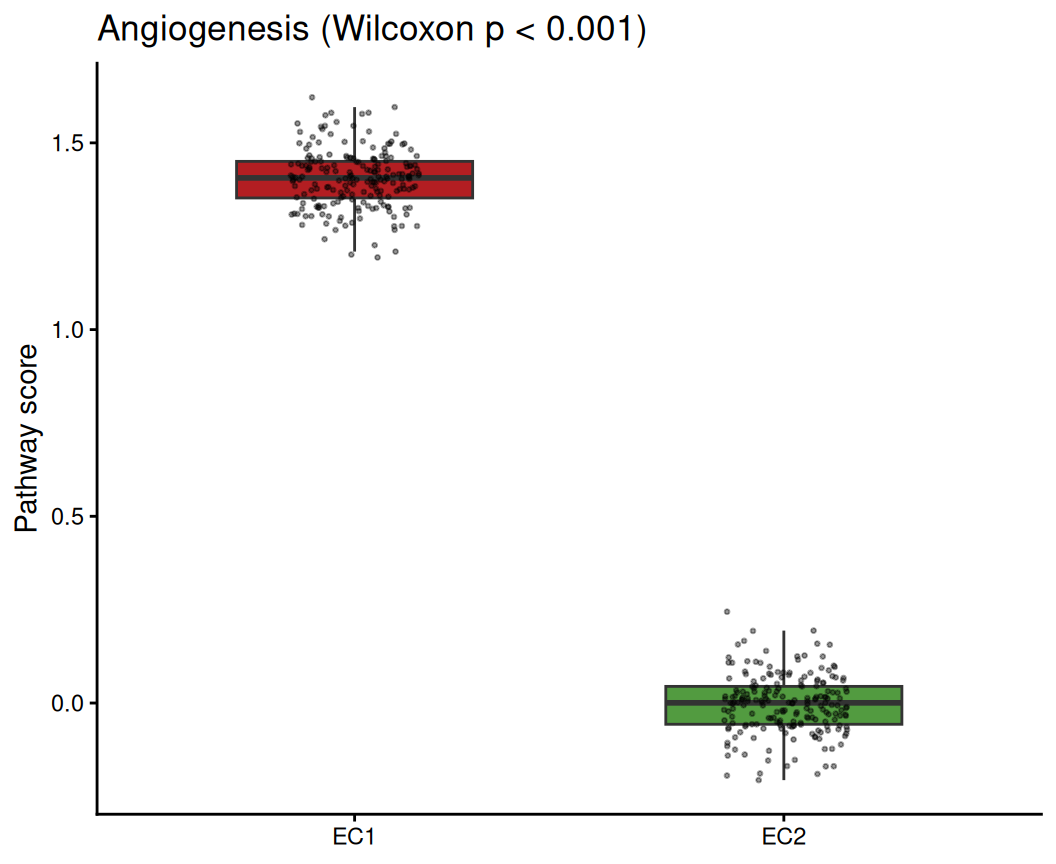
Tip
Practice tips
- Score cells on the normalised data (
GetAssayData(slot = "data")in Seurat), never raw counts. - With real data, run
GSVA::gsva(expr, pathways)on the cells × genes matrix — the heatmap and boxplot halves stay exactly as here. - Two clusters ↔︎ one Wilcoxon test; for more clusters use a Kruskal-Wallis per pathway (
ggpubr::stat_compare_means(method = "kruskal.test")).
Application
Per-cell pathway scoring is the standard read-out when annotating subpopulations (endothelial tips vs phalanx cells, tumour vs stromal fibroblasts). The heatmap reveals which programs define which cluster; the boxplot quantifies one program of interest.
Reference
[1] Xiaofan Lu, et al. FigureYa: A Standardized Visualization Framework for Enhancing Biomedical Data Interpretation and Research Efficiency. iMetaMed. 2025. doi:10.1002/imm3.70005