3D 散点图 (Python)

🤖 AI Skill — Download the Bizard unified skill for your AI assistant ⬇️ Download Skill ZIP

🔌 MCP Server — Let AI agents (Claude Code, Cursor, …) query Bizard live: claude mcp add bizard -- npx @openbiox/bizard-mcp — or the free hosted instance (no install, faster from mainland China): claude mcp add --transport http bizard http://biotree.top:38123/bizard-mcp/mcp 📖 MCP Docs

📖 Cite Bizard — if Bizard helps your research, please cite: Li, K., Zheng, H., Huang, K., et al. (2026). Bizard: A Community-Driven Platform for Accelerating and Enhancing Biomedical Data Visualization. iMetaMed, e70038. 🔗 DOI / BibTeX

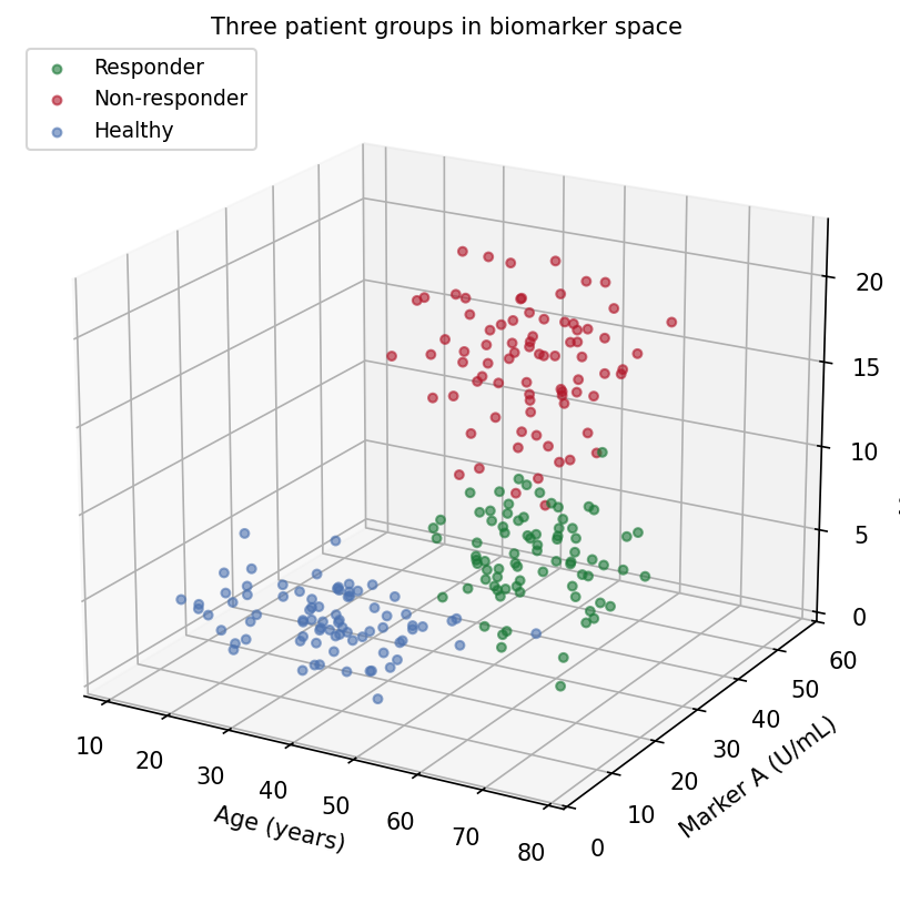
3D 散点图的 Python 对应版本——3D 散点图把每个受试者放到三个定量变量的 \((x, y, z)\) 坐标上，在经典二维散点之上再加一维生物标志物。当组间分离确实存在于三个变量（年龄 x 标志物 x 标志物、细胞大小 x 颗粒度 x 荧光强度）、而二维投影明显压平了结构时，转化医学研究可以用它辅助探索 [1]。

matplotlib 的 mplot3d 负责渲染 [2]。3D 散点易被误读的两个原因：视角决定哪些簇藏在哪些簇后面；深度只靠大小/透明度着色暗示——印刷出来的 3D 图是三维对象的单一固定投影。两者都应作为需要报告的参数对待，就像模型一样。

本教程涵盖两种工作流：

1. 三个患者组的默认视角 3D 散点；
2. 展示同一数据”换角度换结论”的旋转面板。

Example

Setup

• 系统要求：跨平台（Linux/MacOS/Windows）
• 编程语言：Python
• 依赖包：matplotlib、numpy

import matplotlib.pyplot as plt
import numpy as np
from mpl_toolkits.mplot3d import Axes3D  # noqa: F401 (注册 3d 投影)

Data Preparation

我们模拟 240 名受试者的三组（年龄, 标志物 A, 标志物 B）轮廓：应答者年龄较大、标志物居中，非应答者标志物最高，健康供者最低。分离方向经过挑选——有些视角能分开三组，有些视角会把它们压扁。

rng = np.random.default_rng(21)
groups = {
    "Responder":     (np.array([60, 25, 8]),  np.array([8, 6, 2.2]),
                      "#1B7837"),
    "Non-responder": (np.array([48, 40, 15]), np.array([9, 7, 3.0]),
                      "#B2182B"),
    "Healthy":       (np.array([35, 12, 4]),  np.array([10, 4, 1.4]),
                      "#4C72B0"),
}
n_per = 80
data = []
for g, (mu, sd, color) in groups.items():
    xyz = np.column_stack([rng.normal(m, s, n_per)
                           for m, s in zip(mu, sd)])
    data.append((g, xyz, color))

def draw(ax, elev, azim, title):
    for g, xyz, color in data:
        ax.scatter(xyz[:, 0], xyz[:, 1], xyz[:, 2], s=14, alpha=0.6,
                   color=color, label=g, depthshade=True)
    ax.set_xlabel("Age (years)")
    ax.set_ylabel("Marker A (U/mL)")
    ax.set_zlabel("Marker B (ng/mL)")
    ax.view_init(elev=elev, azim=azim)
    ax.set_title(title, fontsize=10, pad=0)
    ax.set_box_aspect((1, 1, 0.8))

Visualization

1. 默认视角

fig = plt.figure(figsize=(7.5, 5.6))
ax = fig.add_subplot(111, projection="3d")
draw(ax, elev=20, azim=-60,
     title="Three patient groups in biomarker space")
ax.legend(loc="upper left", fontsize=9)
fig.tight_layout()
plt.show()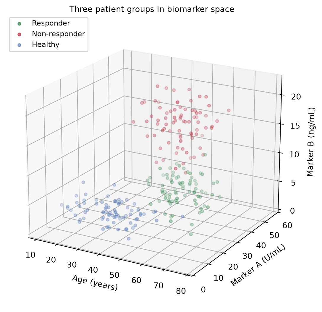

图 1: elev=20、azim=-60 下的三维生物标志物空间：三组占据体积中的不同区域。

2. 旋转面板

fig = plt.figure(figsize=(11.5, 4.8))
for i, (elev, azim, title) in enumerate([
        (20, -60, "View A (elev=20, azim=-60): groups look separable"),
        (2, 55, "View B (elev=2, azim=55): edge-on view obscures depth")]):
    ax = fig.add_subplot(1, 2, i + 1, projection="3d")
    draw(ax, elev=elev, azim=azim, title=title)
fig.suptitle("One dataset, two stories: rotation changes the reading",
             y=1.0)
fig.tight_layout()
plt.show()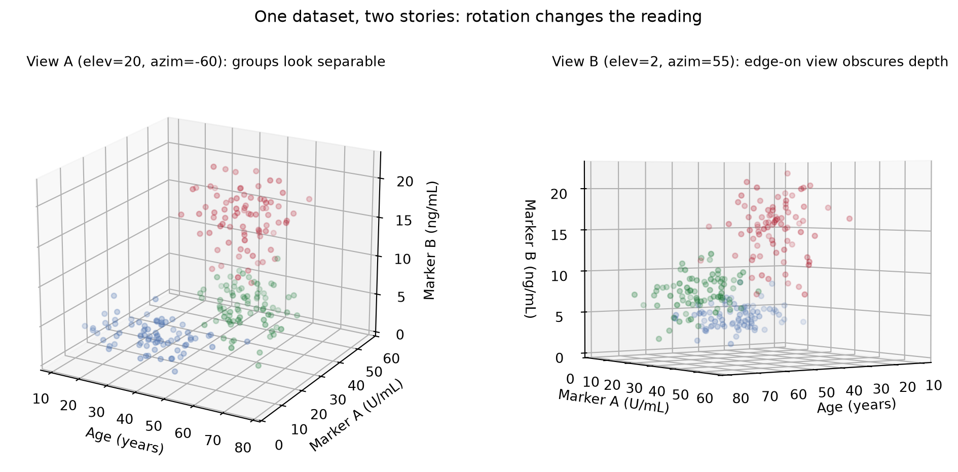

图 2: 同一数据的两个视角：左图的组间分离在右图的侧视中不可得——深度顺序与反转的轴方向都难以判断。

提示实践要点

• 当结论依赖视角时，在图注中报告 elev/azim；否则审稿人无法复现你的分离结果。
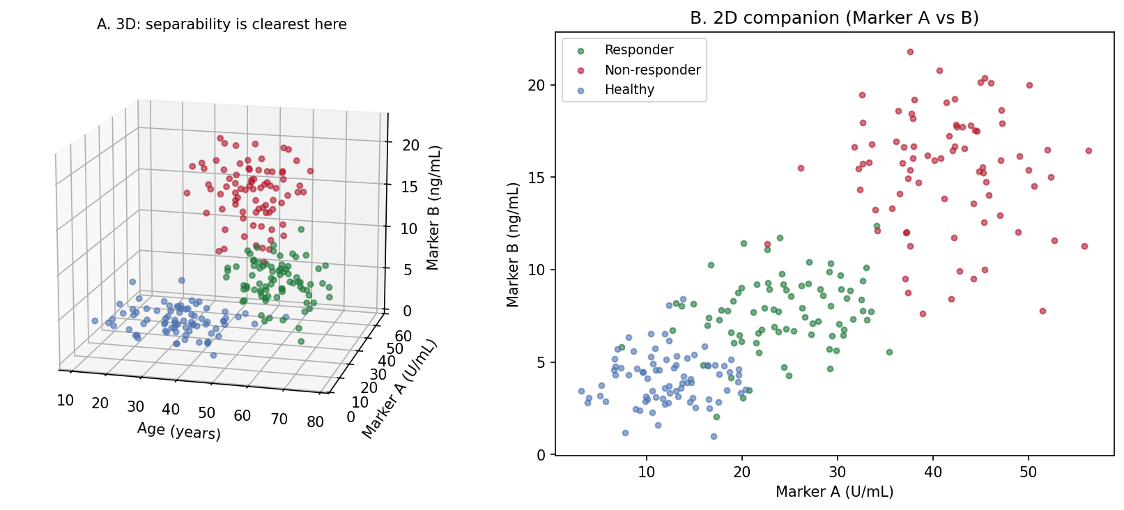
• alpha + depthshade 只是暗示深度——点仍会互相覆盖。降低 alpha、缩小点径可减少错误的遮挡判断。
• 任何定量比较都优先用变量两两的 2D 面板（Application 面板 B）；3D 视图只用来引出它们。
• 用 ax.set_box_aspect() 设定有物理含义的比例，否则量程 3x 的轴会在视觉上碾压量程 1x 的轴。
• 交互旋转（notebook 的 %matplotlib widget、plotly Scatter3d）用于探索；出版导出时固定所选角度。

Application

出版搭配把选定的 3D 视角（A）与最强的 2D 投影（B）并排：3D 面板引出三组结构，2D 面板承载论文统计所对应的可读、可量化的比较。

Reference

[1] Li J, Martens JB. Judging correlation from scatterplots: an evaluation of 3D visualizations. IEEE Trans Vis Comput Graph. 2010;16(6):1027-1036.

[2] Hunter JD. Matplotlib: a 2D graphics environment. Comput Sci Eng. 2007;9(3):90-95. doi:10.1109/MCSE.2007.55