# Install packages
if (!requireNamespace("tidyverse", quietly = TRUE)) {
  install.packages("tidyverse")
}
if (!requireNamespace("viridis", quietly = TRUE)) {
  install.packages("viridis")
}
if (!requireNamespace("patchwork", quietly = TRUE)) {
  install.packages("patchwork")
}
if (!requireNamespace("igraph", quietly = TRUE)) {
  install.packages("igraph")
}
if (!requireNamespace("ggraph", quietly = TRUE)) {
  install.packages("ggraph")
}
if (!requireNamespace("colormap", quietly = TRUE)) {
  install.packages("colormap")
}

# Load packages
library(tidyverse)
library(viridis)
library(patchwork)
library(igraph)
library(ggraph)
library(colormap) Arc Diagram
The arc diagram is a diagram connected by arcs, showing the relationships between nodes.
Example
The figure shows a simple arc diagram. The nodes are neatly arranged at the bottom of the diagram and connected by arcs, forming the main body of the arc diagram.
Setup
System Requirements: Cross-platform (Linux/MacOS/Windows)
Programming Language: R
Dependencies:
ggraph,tidyverse,viridis,patchwork,igraph,colormap
sessioninfo::session_info("attached")─ Session info ───────────────────────────────────────────────────────────────
setting value
version R version 4.6.0 (2026-04-24)
os Ubuntu 24.04.4 LTS
system x86_64, linux-gnu
ui X11
language (EN)
collate C.UTF-8
ctype C.UTF-8
tz UTC
date 2026-05-09
pandoc 3.1.3 @ /usr/bin/ (via rmarkdown)
quarto 1.9.37 @ /usr/local/bin/quarto
─ Packages ───────────────────────────────────────────────────────────────────
package * version date (UTC) lib source
colormap * 0.1.4 2016-11-15 [1] RSPM
dplyr * 1.2.1 2026-04-03 [1] RSPM
forcats * 1.0.1 2025-09-25 [1] RSPM
ggplot2 * 4.0.3.9000 2026-05-04 [1] Github (tidyverse/ggplot2@6870419)
ggraph * 2.2.2 2025-08-24 [1] RSPM
igraph * 2.3.1 2026-05-04 [1] RSPM
lubridate * 1.9.5 2026-02-04 [1] RSPM
patchwork * 1.3.2 2025-08-25 [1] RSPM
purrr * 1.2.2 2026-04-10 [1] RSPM
readr * 2.2.0 2026-02-19 [1] RSPM
stringr * 1.6.0 2025-11-04 [1] RSPM
tibble * 3.3.1 2026-01-11 [1] RSPM
tidyr * 1.3.2 2025-12-19 [1] RSPM
tidyverse * 2.0.0 2023-02-22 [1] RSPM
viridis * 0.6.5 2024-01-29 [1] RSPM
viridisLite * 0.4.3 2026-02-04 [1] RSPM
[1] /home/runner/work/_temp/Library
[2] /opt/R/4.6.0/lib/R/site-library
[3] /opt/R/4.6.0/lib/R/library
* ── Packages attached to the search path.
──────────────────────────────────────────────────────────────────────────────Data Preparation
The data includes custom data, co-authored networks of researchers, and PPI network data exported by Cytoscape software.
# 1.Custom data
# `links` stores edge information, and `nodes` stores node information and node grouping information.
links <- data.frame(
source = c("A", "A", "A", "A", "B", "G", "G", "G", "G"),
  target = c("B", "C", "D", "F", "E", "H", "I", "J", "F")
)
nodes <- data.frame(
  point = c("A", "B", "C", "D", "E", "F", "G", "H", "I", "J"),
  groups = c(
    "group-one", "group-one", "group-one", "group-one", "group-one",
    "group-one", "group-two", "group-two", "group-two", "group-two"
  )
)

head(links)
source target
1 A B
2 A C
3 A D
4 A F
5 B E
6 G Hhead(nodes) point groups
1 A group-one
2 B group-one
3 C group-one
4 D group-one
5 E group-one
6 F group-one# 2.Researchers co-authored network
# Copy the link information to a txt file, read it, and draw the plot.
data_dif <- read.csv("https://bizard-1301043367.cos.ap-guangzhou.myqcloud.com/Arc.txt", header = T, sep = " ")
head(data_dif[,1:5]) from A.Bateman A.Besnard A.Breil A.Cenci
1 A Armero NA NA 1 NA
2 A Bateman NA NA NA NA
3 A Besnard NA NA NA NA
4 A Breil NA NA NA NA
5 A Cenci NA NA NA NA
6 A Chifolleau NA NA NA NA# 3.PPI network node and edge data
# Read PPI network information downloaded from GitHub
data_ppi <- read.csv("https://bizard-1301043367.cos.ap-guangzhou.myqcloud.com/string_interactions_short.tsv_1%20default%20edge.csv", header = TRUE)
head(data_ppi[,c(9,3)]) name combined_score
1 ABCB4 (interacts with) CFTR 0.458
2 ABCB4 (interacts with) CREBBP 0.440
3 ABCB4 (interacts with) ABCC8 0.410
4 ABCB5 (interacts with) CFTR 0.415
5 ABCB5 (interacts with) ABCC8 0.436
6 ABCB5 (interacts with) PROM1 0.786Basic arc diagram
1. Basic arc diagram
# Basic arc diagram
mygraph <- graph_from_data_frame(links, vertices = nodes) # Generate graph structure

p <- ggraph(mygraph, layout = "linear") +
  geom_edge_arc(edge_colour = "black", edge_alpha = 0.3, edge_width = 0.4) +
  geom_node_point(color = "grey", size = 5) +
  geom_node_text(aes(label = name), repel = FALSE, size = 6, nudge_y = -0.15) +
  theme_void() +
  theme(
    legend.position = "none",
    plot.margin = unit(rep(2, 4), "cm")
  )

p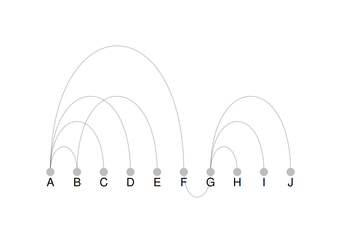
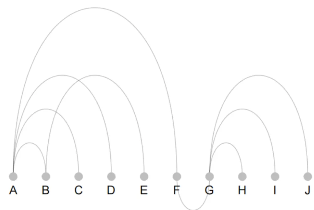
The figure shows the drawing of a basic arc diagram. It has few nodes and edges, so the structure of the arc diagram is simple.
2. Map group information to node colors
# Map group information to node colors
mygraph <- graph_from_data_frame(links, vertices = nodes) # Generated graph
p <- ggraph(mygraph, layout = "linear") +
  geom_edge_arc(edge_colour = "black", edge_alpha = 0.3, edge_width = 0.4) +
  geom_node_point(aes(color = groups), size = 5) +
  geom_node_text(aes(label = name), repel = FALSE, size = 6, nudge_y = -0.15) +
  theme_void() +
  theme(
    legend.position = "none",
    plot.margin = unit(rep(2, 4), "cm")
  )
p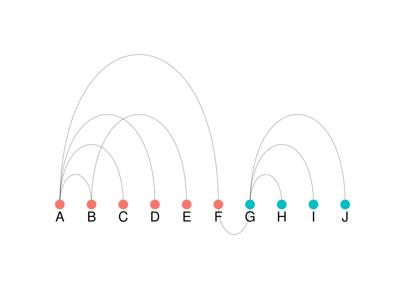
As shown in the figure, color = groups maps grouping information to the color of the nodes, which can be seen intuitively in the arc diagram.
3. Drawing complex graph structures
Typical raw data often contains many nodes and edges, resulting in complex graph structures. When plotting, nodes need to be categorized and sorted, and the size of nodes and edges needs to be measured to display an aesthetically pleasing arc graph. This study uses co-authored network data from researchers.
# Co-authored Network Data Processing and Graphics
# 1.Data layout transformation
connect <- data_dif %>% # connect stores the edge information of the nodes.
  gather(key = "to", value = "value", -1) %>% # Use this method to convert the data excluding the first column into two columns (one column for column names and one column for values).
  mutate(to = gsub("\\.", " ", to)) %>% # Change the column name format from "to" to be consistent with "from".
  na.omit() # Remove NA value

# 2.Node statistics
coauth <- # coauth stores node names and in/out degree information; grouping information will be added later.
  c(as.character(connect$from), as.character(connect$to)) %>%
  as.tibble() %>% # Similar to a data frame type, column names default to "value" —
  group_by(value) %>% # Group by "value"
  summarize(n = n()) # Count the in-degree and out-degree of node names
colnames(coauth) <- c("name", "n") # Change column name

# 3.Grouping nodes
mygraph <- graph_from_data_frame(connect, vertices = coauth, directed = FALSE) # Generate a graph
com <- walktrap.community(mygraph) # Grouping based on the path size of the nodes————
# Add group information to Coauth
coauth <- coauth %>%
  mutate(grp = com$membership) %>% # Add Groups
  arrange(grp) %>% # Sort by group
  mutate(name = factor(name, name))

# 4.Select the top 15 groups
coauth <- coauth[coauth$grp < 16, ]
# Filter connections that appear only in the first 15 sets of points.
connect <- connect %>%
  filter(from %in% coauth$name) %>%
  filter(to %in% coauth$name)

# 5.Generate a graph
mygraph <- graph_from_data_frame(connect, vertices = coauth, directed = FALSE)
# Generate colors by group
mycolor <- colormap(colormap = colormaps$viridis, nshades = max(coauth$grp))
mycolor <- sample(mycolor, length(mycolor))
# ggraph drawing
ggraph(mygraph, layout = "linear") +
  geom_edge_arc(edge_colour = "black", edge_alpha = 0.2, edge_width = 0.3, fold = TRUE) +
  geom_node_point(aes(size = n, color = as.factor(grp), fill = grp), alpha = 0.5) + # Map n and the grouping variable to size and color.
  scale_size_continuous(range = c(0.5, 8)) + # Set size range
  scale_color_manual(values = mycolor) + # Set the group color
  geom_node_text(aes(label = name), angle = 65, hjust = 1, nudge_y = -1.1, size = 2.3) + # Set node labels and skew them to avoid overlap.
  theme_void() + # Remove background table, axis theme
  theme(
    legend.position = "none", # Remove legend
    plot.margin = unit(c(0, 0, 0.4, 0), "null"),
    panel.spacing = unit(c(0, 0, 3.4, 0), "null")
  ) +
  expand_limits(x = c(-1.2, 1.2), y = c(-5.6, 1.2))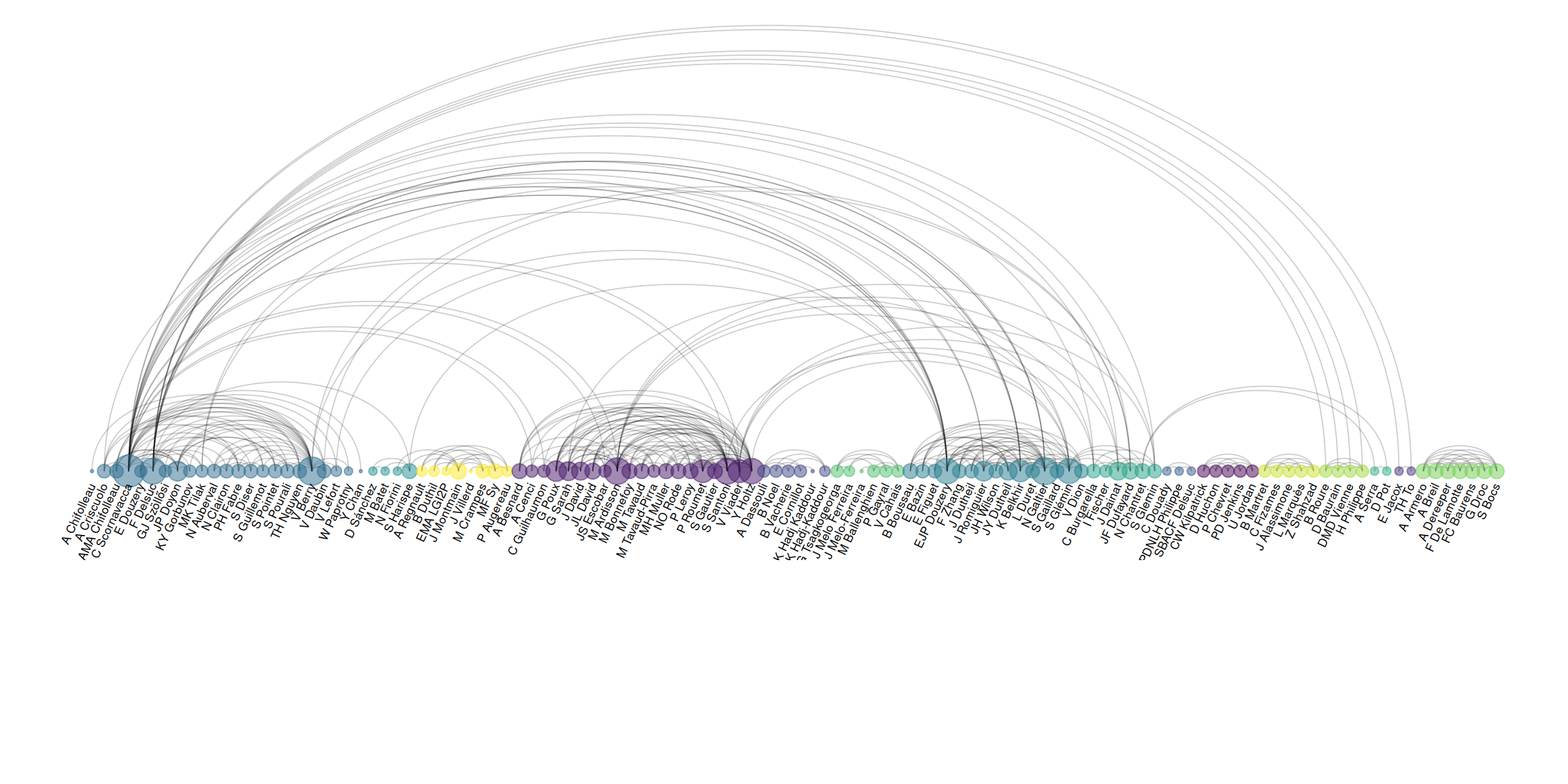
The figure shows an arc diagram drawn based on a complex graph structure. Drawing an arc diagram (or graph in general) requires preprocessing the data into two data frames, one containing node information and the other containing edge information. The data processing steps in this case are as follows:
- Modify the data layout to generate edge information (stored via
connect); - Extract all node information based on the edge information (stored via
coauth); - Group nodes according to
walktrap.community(). Grouping features can be mapped to node colors to display different groups. For aesthetic purposes, sort the grouped nodes; - Select only the preceding groups, and filter the nodes in the preceding
connectgroups; - Generate the graph and use
ggraph()to plot it, selecting colors.
Plotting complex data without grouping or sorting (for comparison)
# No grouping or sorting (comparison)
# 1.Data layout transformation
connect <- data_dif %>% # connect stores the edge information of the nodes.
  gather(key = "to", value = "value", -1) %>% # Use this method to convert the data excluding the first column into two columns (one column for column names and one column for values).
  mutate(to = gsub("\\.", " ", to)) %>% # Change the column name format from "to" to be consistent with "from".
  na.omit() # Remove NA value

# 2.Node statistics
coauth <- # coauth stores node names and in/out degree information; grouping information will be added later.
  c(as.character(connect$from), as.character(connect$to)) %>%
  as.tibble() %>% # Similar to a data frame type, column names default to "value" —
  group_by(value) %>% # Group by "value"
  summarize(n = n()) # Count the in-degree and out-degree of node names
colnames(coauth) <- c("name", "n") # Change column name

# 5.Generate a graph
mygraph <- graph_from_data_frame(connect, vertices = coauth, directed = FALSE)
# ggraph drawing
ggraph(mygraph, layout = "linear") +
  geom_edge_arc(edge_colour = "black", edge_alpha = 0.2, edge_width = 0.3, fold = TRUE) +
  geom_node_point(aes(size = n), alpha = 0.5) + # Map n and the grouping variable to size and color.
  scale_size_continuous(range = c(0.5, 8)) + # Set size range
  geom_node_text(aes(label = name), angle = 65, hjust = 1, nudge_y = -1.1, size = 2.3) + # Set node labels and skew them to avoid overlap.
  theme_void() + # Remove background table, axis theme
  theme(
    legend.position = "none", # Remove legend
    plot.margin = unit(c(0, 0, 0.4, 0), "null"),
    panel.spacing = unit(c(0, 0, 3.4, 0), "null")
  ) +
  expand_limits(x = c(-1.2, 1.2), y = c(-5.6, 1.2))
The image shows an arc graph drawn from complex graph data without grouping and sorting. As you can see, the nodes and arcs are very disorganized, and the content of the arc graph is uninterpretable. Therefore, when drawing arc graphs from complex graph data, it is essential to group and sort the nodes and use color mapping to categorize different points.
4. The thickness of the arc is defined according to the edge weight.
Sometimes the edges of a graph are assigned weights, which can be mapped to the thickness of an arc.
# 1.Edge information is extracted from the PPI data table, and the combined score value is used as the weight.
data_ppi <- data_ppi[, c(9, 3)] # Extract columns 3 and 9
data_ppi$from <- gsub(" \\(.*", "", data_ppi[, 1]) # Extract the left-hand node name of name
data_ppi$to <- gsub(".*\\) ", "", data_ppi[, 1]) # Extract the right-hand node name of name
connect <- data_ppi[, -1] # Remove the first column
connect <- connect[, c(2, 3, 1)] # Place the two columns of information at the beginning (from and to columns).

# 2.Node statistics
coauth <- # coauth stores node names and in/out degree information; grouping information will be added later.
  c(as.character(connect$from), as.character(connect$to)) %>%
  as.tibble() %>% # Similar to a data frame type, column names default to "value" —
  group_by(value) %>% # Group by "value"
  summarize(n = n()) # Count the in-degree and out-degree of node names
colnames(coauth) <- c("name", "n") # Change column name

# 3.Grouping nodes
mygraph <- graph_from_data_frame(connect, vertices = coauth, directed = FALSE) # Generate a graph
com <- walktrap.community(mygraph) # Grouping nodes based on their path length —
## Add group information to Coauth
coauth <- coauth %>%
  mutate(grp = com$membership) %>% # Add Groups
  arrange(grp) %>% # Sort by group
  mutate(name = factor(name, name))

# 4.Select the top 15 groups
coauth <- coauth[coauth$grp < 16, ]
# Filter connections that appear only in the first 15 sets of points.
connect <- connect %>%
  filter(from %in% coauth$name) %>%
  filter(to %in% coauth$name)

# 5.Generate a graph
mygraph <- graph_from_data_frame(connect, vertices = coauth, directed = FALSE)
# Generate colors by group
mycolor <- colormap(colormap = colormaps$viridis, nshades = max(coauth$grp))
mycolor <- sample(mycolor, length(mycolor))
# ggraph drawing
ggraph(mygraph, layout = "linear") +
  geom_edge_arc(aes(edge_width = connect$combined_score), edge_colour = "black", edge_alpha = 0.2, fold = TRUE) +
  geom_node_point(aes(size = n, color = as.factor(grp), fill = grp), alpha = 0.5) + # Map n and the grouping variable to size and color.
  scale_size_continuous(range = c(0.5, 8)) + # Set size range
  scale_color_manual(values = mycolor) + # Set the group color
  geom_node_text(aes(label = name), angle = 65, hjust = 1, nudge_y = -1.1, size = 2.3) + # Set node labels and skew them to avoid overlap.
  theme_void() + # Remove background table, axis theme
  theme(
    legend.position = "none", # Remove legend
    plot.margin = unit(c(0, 0, 0.4, 0), "null"),
    panel.spacing = unit(c(0, 0, 3.4, 0), "null")
  ) +
  expand_limits(x = c(-1.2, 1.2), y = c(-5.6, 1.2))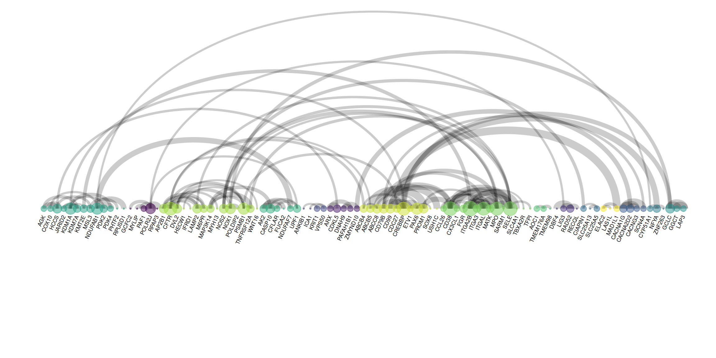
The figure shows an arc graph drawn using PPI edge data. Nodes represent genes, arcs represent relationships between genes, and the thickness of the arcs represents the weight (strength) of the relationships between genes. Unlike the previous figure, the edge information is extracted, and edge_width = connect$combined_score is used in the drawing process to map the weights to the thickness of the arcs.
Applications
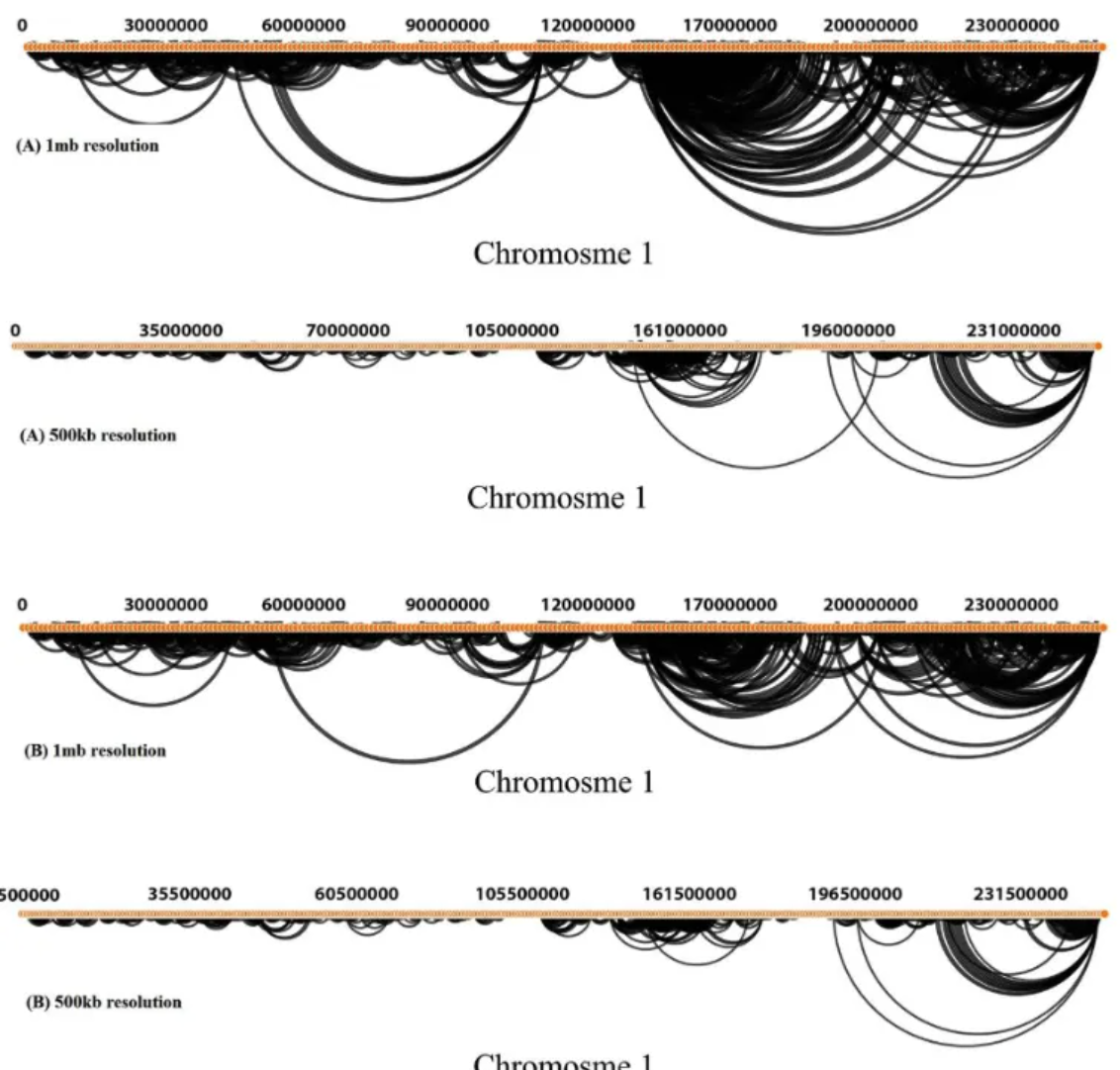
Hi-C interaction arc diagrams across the entire Dixon chromosome at resolutions of 500 Kb and 1 Mb, modeled by GOTHiC. a. Arc diagrams showing interactions at least 50 reads (500 Kb resolution) and 100 reads (1 Mb resolution). b. Arc diagrams of significant interactions. [1]
Reference
[1] KHAKMARDAN S, REZVANI M, POUYAN A A, et al. MHiC, an integrated user-friendly tool for the identification and visualization of significant interactions in Hi-C data[J]. BMC Genomics, 2020,21(1): 225.