# Installing necessary packages
if (!requireNamespace("scRNAtoolVis", quietly = TRUE)) {
  remotes::install_github("junjunlab/scRNAtoolVis")
}
if (!requireNamespace("tidyverse", quietly = TRUE)) {
  install.packages("tidyverse")
}
if (!requireNamespace("ggrepel", quietly = TRUE)) {
  install.packages("ggrepel")
}

# Load packages
library(scRNAtoolVis)
library(tidyverse)
library(ggrepel)FC-FC Scatter Plot
An FC-FC scatter plot (also called a variant volcano plot) compares the fold changes of the same features between two differential contrasts: each point is one gene (or protein, metabolite, …), the X-axis is its log2 fold change in contrast A and the Y-axis its log2 fold change in contrast B. Unlike a volcano plot, which displays one contrast against significance, the FC-FC scatter puts two contrasts side by side, making it easy to identify features that are consistently changed in both contrasts (both axes share the same sign), contrast-specific (changed on only one axis), or discordant (opposite directions) — the typical questions when comparing two datasets, two cell populations, two treatment arms, or discovery and validation cohorts. This tutorial reproduces the chart type covered by the 顶刊图社 series (issue 018); see the Reference section below.
Example
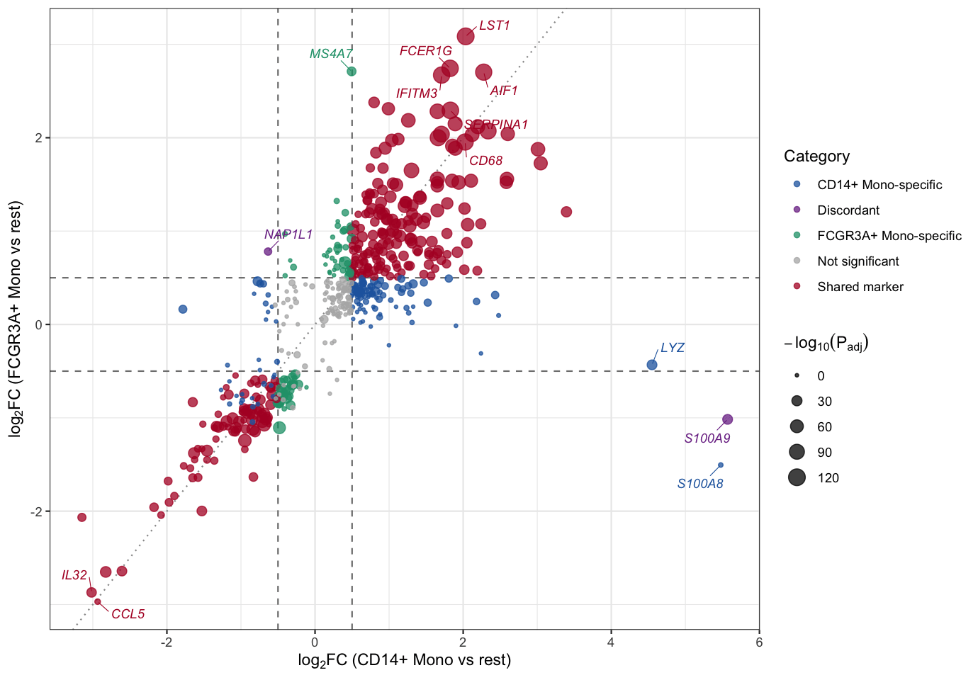
This FC-FC scatter plot compares the marker-gene statistics of two monocyte subsets: the X-axis is the average log2 fold change of each gene in the CD14+ Mono cluster (versus all remaining cells) and the Y-axis is its average log2 fold change in the FCGR3A+ Mono cluster. Points are colored by significance category: shared markers significant in both subsets (red), subset-specific markers (blue/green) and discordant markers with opposite directions (purple); point size encodes the statistical significance. Classical monocyte markers such as S100A8/S100A9 sit at the extreme right on the CD14+ axis (S100A9 is even flagged discordant because its FCGR3A+ fold change is significantly negative), MS4A7 deviates upward (FCGR3A+ Mono specific), while a large group along the diagonal (LST1, FCER1G, AIF1, CD68, …) are shared monocyte markers.
Setup
System Requirements: Cross-platform (Linux/MacOS/Windows)
Programming Language: R
Dependencies:
scRNAtoolVis;tidyverse;ggrepel
Data Preparation
The example uses pbmc.markers, the PBMC single-cell marker-gene table shipped with the scRNAtoolVis package (9 clusters, 5,921 rows of marker statistics). Each row reports one gene’s differential expression statistics in one cluster versus all remaining cells (avg_log2FC, p_val_adj, pct.1, pct.2, …). We compare the two monocyte subsets — CD14+ Mono and FCGR3A+ Mono — by joining their marker statistics gene by gene, which gives two “contrasts” of the same feature set.
# Load the PBMC marker gene table
data("pbmc.markers")

# Marker statistics of the two monocyte subsets
cd14 <- pbmc.markers |>
  filter(cluster == "CD14+ Mono") |>
  select(gene, avg_log2FC, p_val_adj)

fcgr3a <- pbmc.markers |>
  filter(cluster == "FCGR3A+ Mono") |>
  select(gene, avg_log2FC, p_val_adj)

# Join by gene: 546 genes are markers in both subsets
fc_fc <- inner_join(cd14, fcgr3a, by = "gene", suffix = c("_cd14", "_fcgr3a"))

# Classify each gene and compute the plotting score
fc_cut <- 0.5
p_cut <- 0.05
fc_fc <- fc_fc |>
  mutate(
    sig_cd14 = p_val_adj_cd14 < p_cut & abs(avg_log2FC_cd14) >= fc_cut,
    sig_fcgr3a = p_val_adj_fcgr3a < p_cut & abs(avg_log2FC_fcgr3a) >= fc_cut,
    category = case_when(
      sig_cd14 & sig_fcgr3a & sign(avg_log2FC_cd14) == sign(avg_log2FC_fcgr3a) ~ "Shared marker",
      sig_cd14 & sig_fcgr3a ~ "Discordant",
      sig_cd14 ~ "CD14+ Mono-specific",
      sig_fcgr3a ~ "FCGR3A+ Mono-specific",
      TRUE ~ "Not significant"
    ),
    neglog10p = -log10(pmax(p_val_adj_cd14, p_val_adj_fcgr3a))
  )

# View data
head(fc_fc)
gene avg_log2FC_cd14 p_val_adj_cd14 avg_log2FC_fcgr3a p_val_adj_fcgr3a
1 S100A9 5.570063 0.000000e+00 -1.0166902 1.344914e-27
2 S100A8 5.477394 0.000000e+00 -1.5053622 1.544192e-01
3 FCN1 3.394219 0.000000e+00 1.2064489 4.815941e-32
4 TYROBP 3.046798 4.375406e-280 1.7261132 4.059108e-65
5 CST3 3.009788 7.593974e-265 1.8764843 3.274775e-70
6 LYZ 4.549466 1.467924e-263 -0.4324426 2.513754e-27
sig_cd14 sig_fcgr3a category neglog10p
1 TRUE TRUE Discordant 26.8713054
2 TRUE FALSE CD14+ Mono-specific 0.8112986
3 TRUE TRUE Shared marker 31.3173189
4 TRUE TRUE Shared marker 64.3915694
5 TRUE TRUE Shared marker 69.4848185
6 TRUE FALSE CD14+ Mono-specific 26.5996772Note: For your own data the input is simply two differential analysis tables (for example DESeq2, limma or edgeR results), each containing at least a feature name and a log2 fold change column; join them by feature name before plotting.
Visualization
1. Basic Plot
The basic version draws every gene as a point, with dashed threshold lines for the fold change cutoff and a dotted diagonal for reference. Points on the diagonal change equally in both contrasts.
ggplot(fc_fc, aes(avg_log2FC_cd14, avg_log2FC_fcgr3a)) +
  geom_hline(yintercept = c(-fc_cut, fc_cut), linetype = "dashed", color = "grey50") +
  geom_vline(xintercept = c(-fc_cut, fc_cut), linetype = "dashed", color = "grey50") +
  geom_abline(slope = 1, intercept = 0, linetype = "dotted", color = "grey60") +
  geom_point(color = "#2166AC", size = 1.8, alpha = 0.7) +
  labs(x = expression(log[2]*FC~"(CD14+ Mono vs rest)"),
       y = expression(log[2]*FC~"(FCGR3A+ Mono vs rest)")) +
  theme_bw()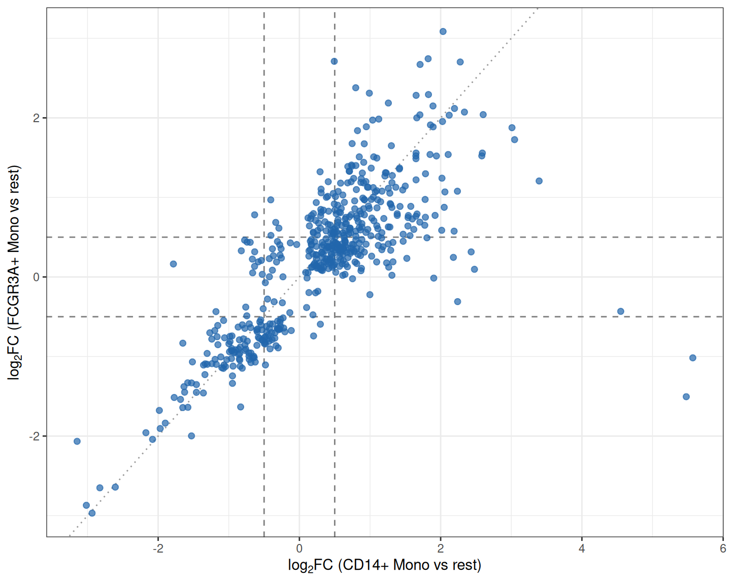
2. Color by Category
Coloring genes by which contrast(s) they are significant in turns the scatter into a readable decision chart: shared markers, subset-specific markers and discordant markers each get their own color.
category_colors <- c(
  "Shared marker" = "#B2182B",
  "Discordant" = "#7B3294",
  "CD14+ Mono-specific" = "#2166AC",
  "FCGR3A+ Mono-specific" = "#1B9E77",
  "Not significant" = "grey70"
)

ggplot(fc_fc, aes(avg_log2FC_cd14, avg_log2FC_fcgr3a)) +
  geom_hline(yintercept = c(-fc_cut, fc_cut), linetype = "dashed", color = "grey50") +
  geom_vline(xintercept = c(-fc_cut, fc_cut), linetype = "dashed", color = "grey50") +
  geom_point(aes(color = category), size = 2, alpha = 0.75) +
  scale_color_manual(values = category_colors) +
  labs(x = expression(log[2]*FC~"(CD14+ Mono vs rest)"),
       y = expression(log[2]*FC~"(FCGR3A+ Mono vs rest)"),
       color = "Category") +
  theme_bw()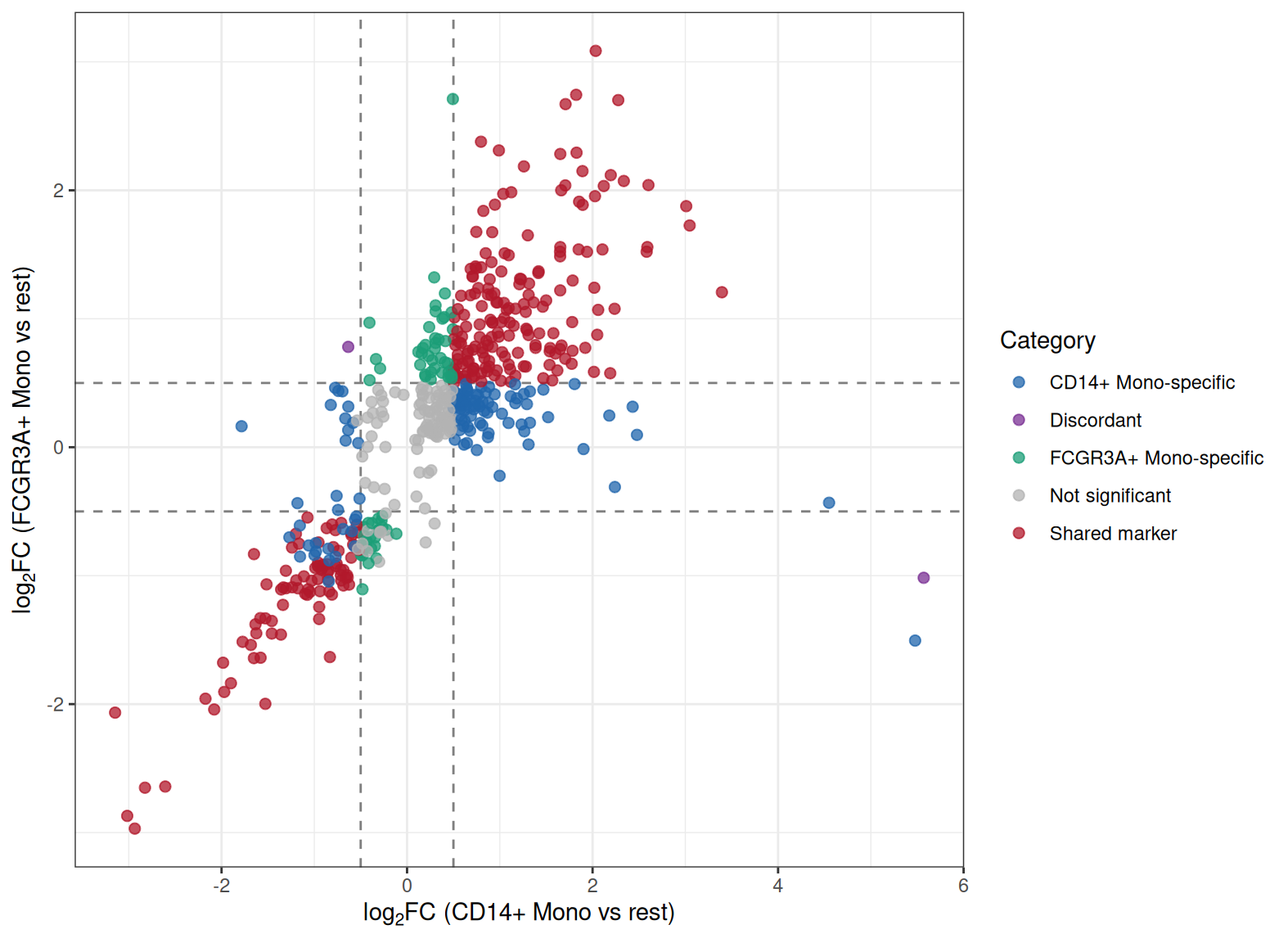
Tip
Key Parameters:
-
fc_cut: The fold change threshold. Withfc_cut = 0.5a gene counts as changed when its |log2FC| ≥ 0.5 on an axis; adjust it to your data scale. -
p_cut: The adjusted P value cutoff used to call significance (0.05 here); it separates real markers from noise when assigning categories.
3. Point Size and Gene Labels
Encoding statistical significance as point size and labeling the most interesting genes completes the plot: extremes on either axis, shared markers with the strongest joint evidence, and the discordant genes.
# Curated label set: discordant genes, extremes on both axes and top shared markers
label_genes <- bind_rows(
  fc_fc |> filter(category == "Discordant") |>
    slice_max(abs(avg_log2FC_cd14 - avg_log2FC_fcgr3a), n = 3),
  fc_fc |> slice_max(abs(avg_log2FC_cd14), n = 3),
  fc_fc |> slice_max(abs(avg_log2FC_fcgr3a), n = 3),
  fc_fc |> filter(gene == "MS4A7"),
  fc_fc |> filter(category == "Shared marker") |>
    slice_max(neglog10p + pmin(abs(avg_log2FC_cd14), abs(avg_log2FC_fcgr3a)), n = 6)
) |>
  distinct(gene, .keep_all = TRUE)

ggplot(fc_fc, aes(avg_log2FC_cd14, avg_log2FC_fcgr3a)) +
  geom_hline(yintercept = c(-fc_cut, fc_cut), linetype = "dashed", color = "grey50") +
  geom_vline(xintercept = c(-fc_cut, fc_cut), linetype = "dashed", color = "grey50") +
  geom_abline(slope = 1, intercept = 0, linetype = "dotted", color = "grey60") +
  geom_point(aes(color = category, size = neglog10p), alpha = 0.75) +
  scale_color_manual(values = category_colors) +
  scale_size_continuous(range = c(0.8, 5), name = expression(-log[10](P[adj]))) +
  geom_text_repel(data = label_genes, aes(label = gene, color = category),
                  size = 3.1, fontface = "italic", max.overlaps = 40,
                  box.padding = 0.55, segment.size = 0.25,
                  show.legend = FALSE, seed = 1) +
  labs(x = expression(log[2]*FC~"(CD14+ Mono vs rest)"),
       y = expression(log[2]*FC~"(FCGR3A+ Mono vs rest)"),
       color = "Category") +
  theme_bw()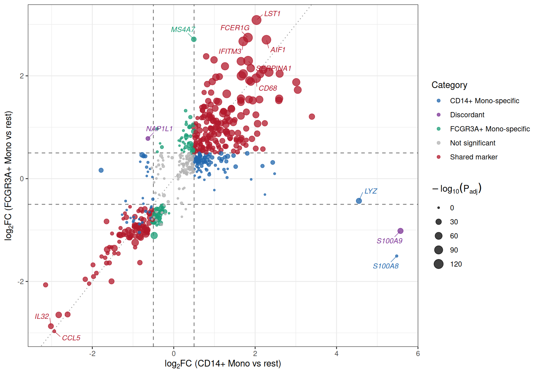
Figure 3 labels the discordant genes S100A9 and NAP1L1, the extreme right-hand genes S100A8 and LYZ on the CD14+ axis, MS4A7 (FCGR3A+ Mono specific), and a block of shared markers (LST1, FCER1G, IFITM3, CD68, AIF1, …) along the diagonal; CCL5 and IL32 sit in the corner where both subsets are consistently depleted. In a two-dataset comparison the same layout would highlight genes consistently changed in both cohorts versus cohort-specific hits.
Applications
The FC-FC scatter plot is widely used when two differential contrasts should be compared feature by feature:
- Two cell populations, tissues or conditions from the same experiment (as in the example above).
- Discovery and validation cohorts, or two independent datasets of the same disease — consistent hits lie near the diagonal.
- Two treatment arms tested against the same control — quadrant analysis separates shared response programs from arm-specific effects.
- Cross-omics comparisons, e.g. transcriptome versus proteome fold changes.
To apply it to your own data, run the differential analysis of each contrast separately, join the two result tables by feature name, and reuse the code above; only the file names and column names need to change.
Reference
[1] 顶刊图社 | 第018期:FC-FC散点图(变异火山图). WeChat article. http://mp.weixin.qq.com/s?__biz=MzU5NjE2ODU0OQ==&mid=2247483956&idx=1&sn=627480882a5c4423980fdefeea18e225
[2] Zhang J. scRNAtoolVis: Making single-cell RNA-seq visualization easier and better. https://github.com/junjunlab/scRNAtoolVis (source of the pbmc.markers dataset).