Manhattan & QQ Plot (Julia)

🤖 AI Skill — Download the Bizard unified skill for your AI assistant ⬇️ Download Skill ZIP

🔌 MCP Server — Let AI agents (Claude Code, Cursor, …) query Bizard live: claude mcp add bizard -- npx @openbiox/bizard-mcp — or the free hosted instance (no install, faster from mainland China): claude mcp add --transport http bizard http://biotree.top:38123/bizard-mcp/mcp 📖 MCP Docs

📖 Cite Bizard — if Bizard helps your research, please cite: Li, K., Zheng, H., Huang, K., et al. (2026). Bizard: A Community-Driven Platform for Accelerating and Enhancing Biomedical Data Visualization. iMetaMed, e70038. 🔗 DOI / BibTeX

A Manhattan plot lines up variants along the genome (x = chromosome position, y = −log10 p) so association peaks rise above the null skyline; the QQ plot compares the observed p distribution with uniform expectation. Julia has no maintained Manhattan helper, so the plot is assembled from two scatter! layers with per-chromosome cumulative offsets.

Example

Setup

• System Requirements: Cross-platform (Linux/MacOS/Windows)
• Programming Language: Julia
• Dependencies: CairoMakie, DataFrames, Statistics

using CairoMakie
using DataFrames
using Statistics
using Random

Data Preparation

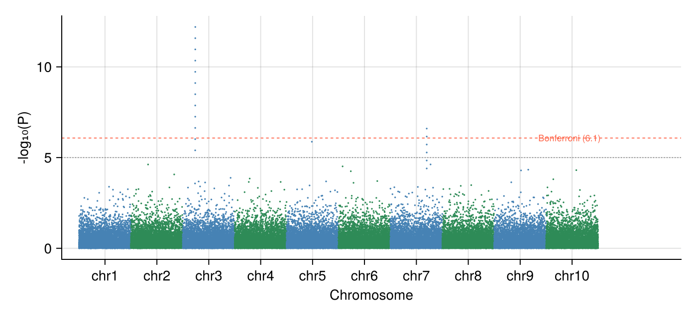
We simulate 60,000 SNPs over 10 chromosomes under the null (uniform p) and inject one association peak on chromosome 3 plus a smaller one on chromosome 7.

Random.seed!(131)

snps_per_chr = 6_000
chr_n = 10
rows = []
for chr in 1:chr_n
    p = rand(snps_per_chr)                      # uniform under the null
    if chr == 3
        p[1500:1511] .= 10.0 .^ (-range(5.4, 12.2; length = 12))
    elseif chr == 7
        p[4200:4205] .= 10.0 .^ (-range(4.4, 6.6; length = 6))
    end
    push!(rows, DataFrame(CHR = chr,
                          POS = sort(rand(snps_per_chr) .* 6_000),
                          P = p))
end
gwas = vcat(rows...)
gwas.MinusLogP = .-log10.(gwas.P)

offsets = DataFrame(CHR = 1:chr_n, Off = (0:chr_n-1) .* 6_000)
pos_range = combine(groupby(gwas, :CHR),
                    :POS => minimum => :Min, :POS => maximum => :Max)
pos_range.PosMid = (pos_range.Min .+ pos_range.Max) ./ 2 .+ offsets.Off
gwas.PosCum = gwas.POS + [offsets.Off[c] for c in gwas.CHR]
BONF = -log10(0.05 / nrow(gwas))
SUGG = -log10(1e-5)

5.0

Visualization

Classic Manhattan Plot

Alternating per-chromosome colours keep neighbours separable; Bonferroni and suggestive thresholds run as horizontal guides.

chr_colors = [c % 2 == 1 ? :steelblue : :seagreen for c in gwas.CHR]

fig = Figure(size = (700, 320))
ax = Axis(fig[1, 1], xlabel = "Chromosome", ylabel = "-log₁₀(P)")
scatter!(ax, gwas.PosCum, gwas.MinusLogP; markersize = 2.4,
         color = chr_colors, strokewidth = 0)
hlines!(ax, [BONF]; color = :tomato, linestyle = :dash, linewidth = 0.9)
hlines!(ax, [SUGG]; color = :gray50, linestyle = :dot, linewidth = 0.9)
text!(ax, nrow(gwas) * 1.005, BONF; text = "Bonferroni ($(round(BONF; digits = 1)))",
      fontsize = 9, color = :tomato, align = (:right, :center))
ax.xticks = (pos_range.PosMid, ["chr$c" for c in pos_range.CHR])
xlims!(ax, -2_000, nrow(gwas) * 1.16)
hidespines!(ax, :t, :r)
fig

Figure 1: Manhattan plot of the simulated GWAS with significance guides

QQ Plot with Inflation Factor

Ordered observed −log10 p against expected uniform quantiles; the median χ²-style ratio summarizes inflation (here ~1.0 by construction).

obs = sort(gwas.MinusLogP; rev = true)
m = length(obs)
expected = -log10.((1:m) ./ (m + 1))
inflation = median(-log.(10, gwas.P)) / median(-log.(10, rand(m))) # ≈ 1 under uniform p

fig = Figure(size = (430, 430))
ax = Axis(fig[1, 1], xlabel = "Expected -log₁₀(P)",
          ylabel = "Observed -log₁₀(P)")
scatter!(ax, expected, obs; markersize = 2.6, color = (:steelblue, 0.6),
         strokewidth = 0)
lim = maximum(expected) * 1.05
lines!(ax, [0, lim], [0, lim]; color = :gray40, linewidth = 0.9)
text!(ax, 0.08, lim * 0.93; text = "λ ≈ $(round(inflation; digits = 2))",
      fontsize = 11)
xlims!(ax, 0, lim); ylims!(ax, 0, lim)
hidespines!(ax, :t, :r)
fig

Figure 2: QQ plot of GWAS p-values

References

1. Turner, S., et al. (2011). Quality Control for Population Association Studies. PLoS Currents, 3, RRN1222.
2. Danisch, S., & Krumbiegel, J. (2021). Makie.jl: Flexible high-performance data visualization for Julia. Journal of Open Source Software, 6(65), 3349.