Complex Heatmap (Python)

🤖 AI Skill — Download the Bizard unified skill for your AI assistant ⬇️ Download Skill ZIP

🔌 MCP Server — Let AI agents (Claude Code, Cursor, …) query Bizard live: claude mcp add bizard -- npx @openbiox/bizard-mcp — or the free hosted instance (no install, faster from mainland China): claude mcp add --transport http bizard http://biotree.top:38123/bizard-mcp/mcp 📖 MCP Docs

📖 Cite Bizard — if Bizard helps your research, please cite: Li, K., Zheng, H., Huang, K., et al. (2026). Bizard: A Community-Driven Platform for Accelerating and Enhancing Biomedical Data Visualization. iMetaMed, e70038. 🔗 DOI / BibTeX

A complex heatmap clusters a matrix and stacks annotation layers (cohort, sex, subtype) beside it, turning an expression table into a single self-contained figure. seaborn.clustermap covers the basics; PyComplexHeatmap adds the publication-grade annotation system — categorical tracks, per-track legends, and split clustering — used across omics papers.

Example

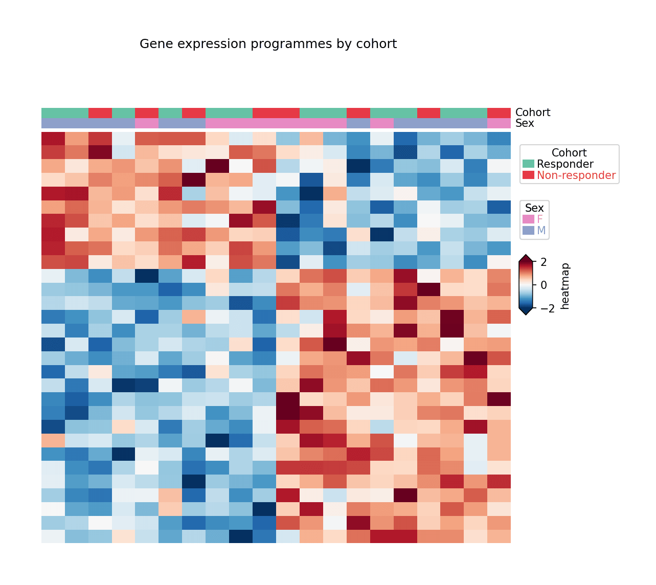
Setup

• System Requirements: Cross-platform (Linux/MacOS/Windows)
• Programming Language: Python
• Dependencies: matplotlib, pandas, numpy, PyComplexHeatmap

import matplotlib.pyplot as plt
import pandas as pd
import numpy as np
from PyComplexHeatmap import ClusterMapPlotter, HeatmapAnnotation, anno_simple

Data Preparation

We simulate a 30-gene × 20-sample expression matrix from two expression programmes plus cohort/sex sample annotations, z-scaled per gene.

np.random.seed(181)

genes = [f'GENE{i:02d}' for i in range(1, 31)]
samples = [f'S{i:02d}' for i in range(1, 21)]
cohort = np.random.choice(['Responder', 'Non-responder'], 20, p=[0.5, 0.5])
sex = np.random.choice(['F', 'M'], 20)

prog1 = np.outer(np.r_[np.ones(10), np.zeros(20)],
                 np.r_[np.full(10, 1.4), np.zeros(10)])
prog2 = np.outer(np.r_[np.zeros(10), np.ones(20)],
                 np.r_[np.zeros(10), np.full(10, 1.2)])
expr = prog1 + prog2 + np.random.normal(0, 0.5, (30, 20))
expr = (expr - expr.mean(axis=1, keepdims=True)) / expr.std(axis=1, keepdims=True)

mat = pd.DataFrame(expr, index=genes, columns=samples)
col_meta = pd.DataFrame({'Cohort': cohort, 'Sex': sex}, index=samples)

Visualization

Clustered Heatmap with Sample Annotations

HeatmapAnnotation stacks categorical tracks above the matrix; ClusterMapPlotter clusters rows and columns and builds the per-track legends automatically.

col_ha = HeatmapAnnotation(
    Cohort=anno_simple(col_meta.Cohort, colors={'Responder': '#66c2a5',
                                                'Non-responder': '#e63946'}),
    Sex=anno_simple(col_meta.Sex, colors={'F': '#e78ac3', 'M': '#8da0cb'}),
    axis=1, verbose=0)

plt.figure(figsize=(8, 6.5))
cm = ClusterMapPlotter(data=mat, top_annotation=col_ha,
                       col_cluster=True, row_cluster=True,
                       show_colnames=False, show_rownames=False,
                       cmap='RdBu_r', vmin=-2, vmax=2, center=0,
                       xticklabels=False, yticklabels=False,
                       rasterized=True, verbose=0)
plt.suptitle('Gene expression programmes by cohort', y=1.02, fontsize=12)
plt.show()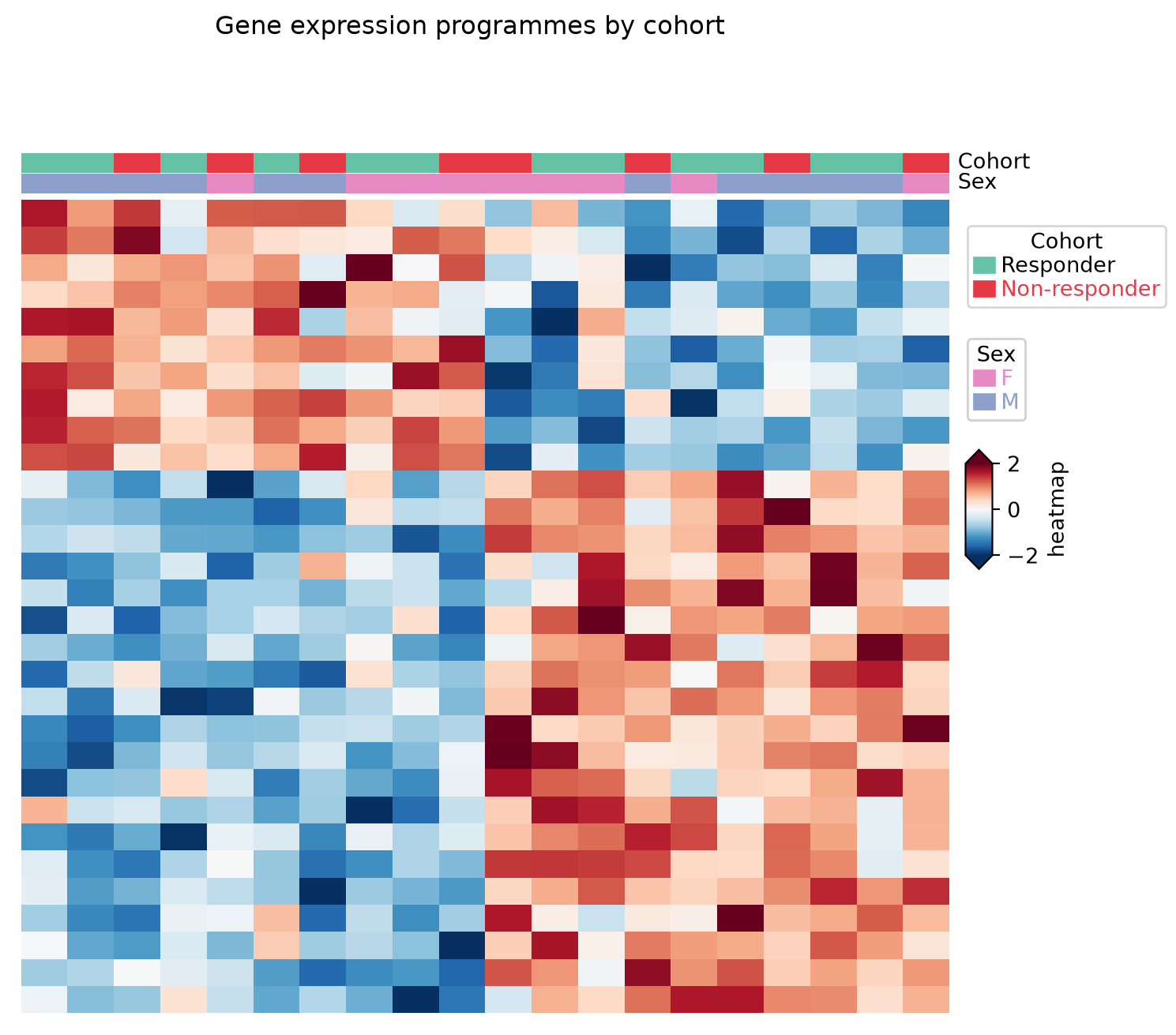

Figure 1: Clustered expression heatmap with cohort and sex annotations

With Gene Labels

At 30 rows a compact font keeps every gene name legible while the two expression programmes stay visible as annotation-separated blocks.

plt.figure(figsize=(8, 6.5))
cm = ClusterMapPlotter(data=mat, top_annotation=col_ha,
                       col_cluster=True, row_cluster=True,
                       show_colnames=False, show_rownames=True,
                       row_names_side='right',
                       yticklabels_kws=dict(labelsize=7),
                       cmap='RdBu_r', vmin=-2, vmax=2, center=0,
                       rasterized=True, verbose=0)
plt.show()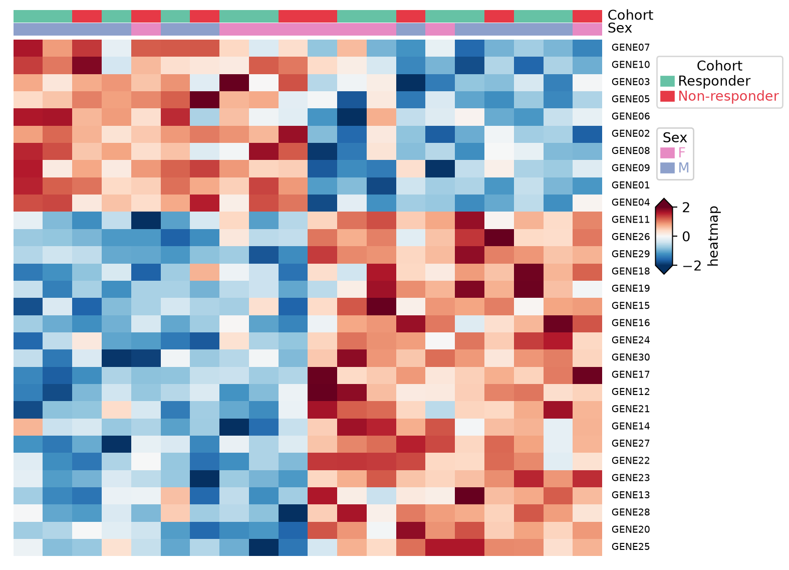

Figure 2: Clustered heatmap with per-gene row labels

References

1. Zhang, W. (2023). PyComplexHeatmap: A Python package to visualize complex heatmaps. https://ding-lab.github.io/PyComplexHeatmap/
2. Gu, Z., Eils, R., & Schlesner, M. (2016). Complex heatmaps reveal patterns and correlations in multidimensional genomic data. Bioinformatics, 32(18), 2847-2849.