Nomogram

Authors

[Editor] Xinhe Lu;

[Contributors] Hu Zheng.

Simply put, a nomogram graphically displays the results of logistic regression or Cox regression. It uses the regression coefficient of each independent variable to develop a scoring criteria, assigning a score to each independent variable value. A total score is then calculated for each patient, and a conversion function is used to convert this score into the probability of a specific outcome for that patient.

Common nomogram names mainly consist of three parts: 1. The name of the variable in the prediction model: for example, “stage,” “gender,” and “age” in the figure. Each variable is marked with a scale on the line segment, indicating the range of values for that variable. The length of the line segment reflects the degree of influence of that factor on the outcome event. 2. Score: This includes individual scores (“β(X-m) terms” in the figure) and a total score (“Total score”). The individual scores represent the scores of each variable at different values, while the total score is the sum of all variable scores. 3. Predicted probability: for example, “mean status” represents the probability of death.

Example

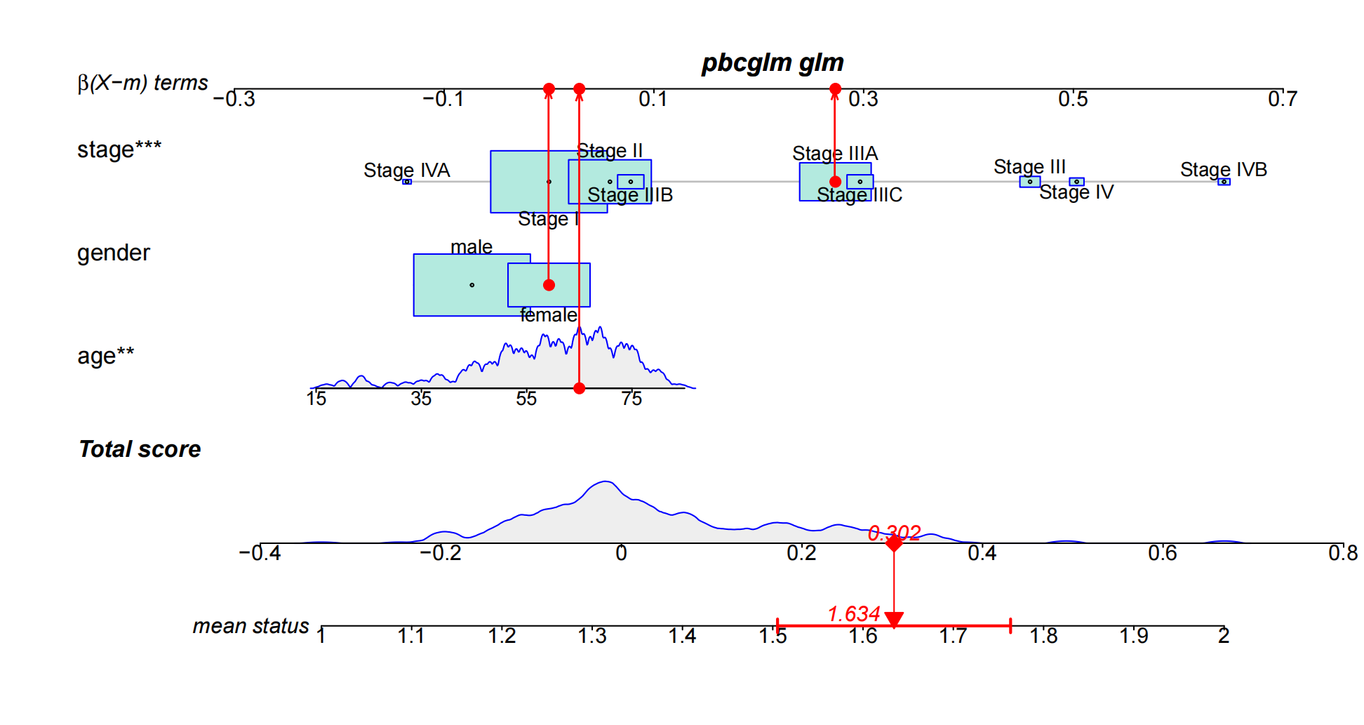
As indicated by the red arrows, find the individual scores for each variable for this patient. Finally, add up the individual scores for all variables to obtain the patient’s total score. Based on this total score, draw a vertical line downward to determine the patient’s risk of invasive lung adenocarcinoma.

Setup

System Requirements: Cross-platform (Linux/MacOS/Windows)
Programming language: R
Dependent packages: readr, rms, survival, regplot

# Installing packages
if (!requireNamespace("readr", quietly = TRUE)) {
  install.packages("readr")
}
if (!requireNamespace("rms", quietly = TRUE)) {
  install.packages("rms")
}
if (!requireNamespace("survival", quietly = TRUE)) {
  install.packages("survival")
}
if (!requireNamespace("regplot", quietly = TRUE)) {
  install.packages("regplot")
}

# Load packages
library(readr)
library(rms)
library(survival)
library(regplot)

Data Preparation

The data were downloaded from the Phenotype file of the GDC TCGA Liver Cancer (LIHC) database in the Xena browser [2].

## Loading data
clinical <- readr::read_tsv("https://bizard-1301043367.cos.ap-guangzhou.myqcloud.com/TCGA-LIHC.clinical.tsv")
LIHC <- cbind(clinical$sample,clinical[,c('gender.demographic',
                                             'vital_status.demographic',
                                             'days_to_death.demographic',
                                             'age_at_index.demographic',
                                             'ajcc_pathologic_stage.diagnoses')])
colnames(LIHC) <- c('bcr_patient_barcode','gender','status','time','age','stage')
table(LIHC$status)


       Alive         Dead Not Reported 
         265          172            2

LIHC <- LIHC[LIHC$status != 'Not Reported',]
LIHC$status <- as.numeric(ifelse(LIHC$status=='Dead','2','1') ) # Death is 2 in nomogram

Visualization

1. Basic Nomogram

The basic nomogram shows the results of modeling survival status (status) with age (age), sex (gender), and disease stage (stage) using a generalized linear model.

# Basic Nomogram
dd=datadist(LIHC)
options(datadist="dd")
## Build a logist model and draw a nomogram
f1 <- lrm(status ~ age + gender + stage , data =  LIHC)
nom <- nomogram(f1, fun=plogis, lp=F, funlabel="Risk")
plot(nom)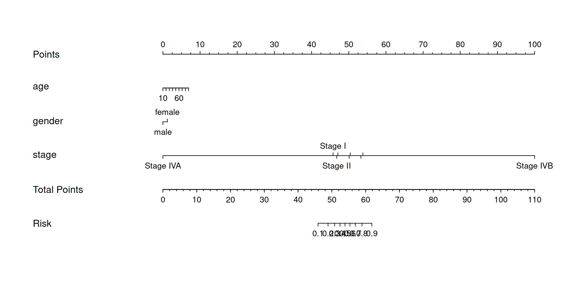

We can also use the nomogram to show the results of the Cox regression model for modeling survival time (time), survival status (status) with age (age), gender (gender), and disease stage (stage).

## Constructing a COX proportional hazards model
f2 <- psm(Surv(time,status) ~ age+gender+stage,data =  LIHC, dist='lognormal')
med <- Quantile(f2) # Calculate median survival time
surv <- Survival(f2) # Constructing a survival probability function
## Draw a nomogram of the median survival time of COX regression
nom <- nomogram(f2, fun=function(x) med(lp=x),funlabel="Median Survival Time")
plot(nom)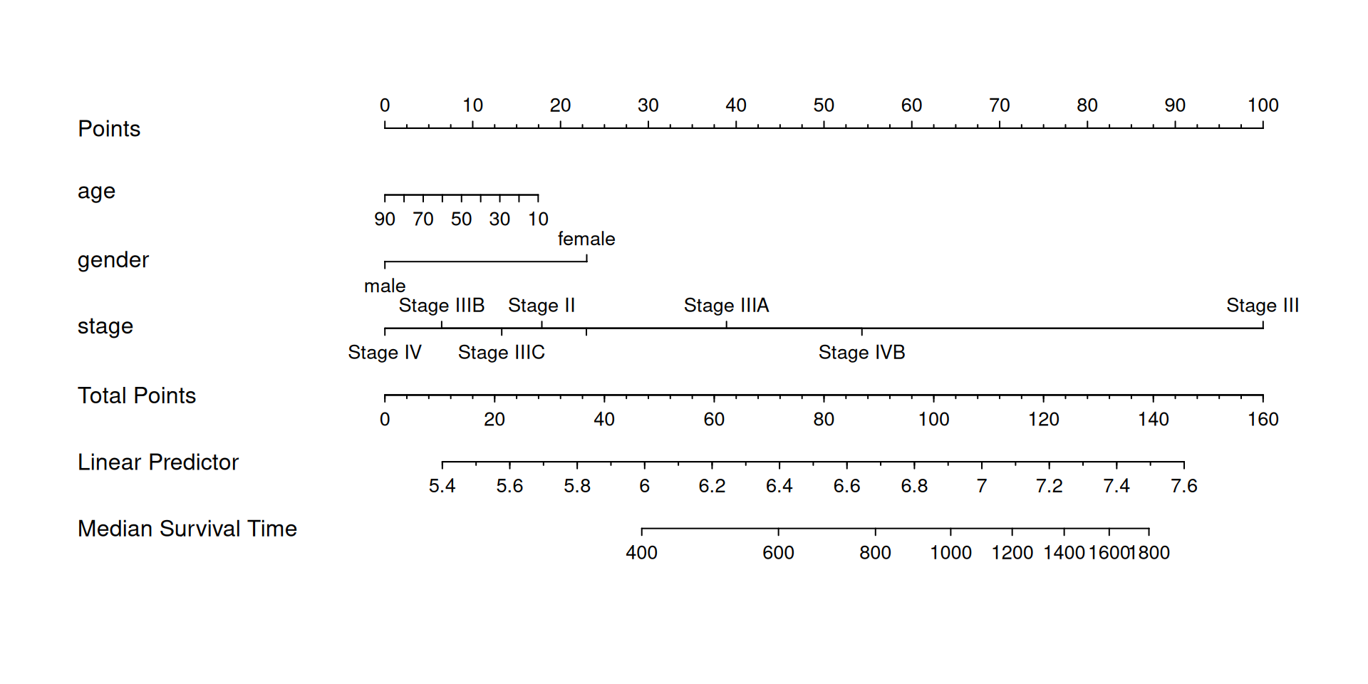

Figure 2: Constructing a COX proportional hazards model

We can also plot the predicted 3-year-5-year-survival probabilities using a nomogram.

## The time unit of LIHC data is "days". Here we plot the 3-year and 5-year survival probabilities.
nom <- nomogram(f2, fun=list(function(x) surv(1095, x),
                             function(x) surv(1825, x),
                             function(x) med(lp=x)),
                funlabel=c("3-year Survival Probability", "5-year Survival Probability","Median Survival Time"))
plot(nom, xfrac=.2)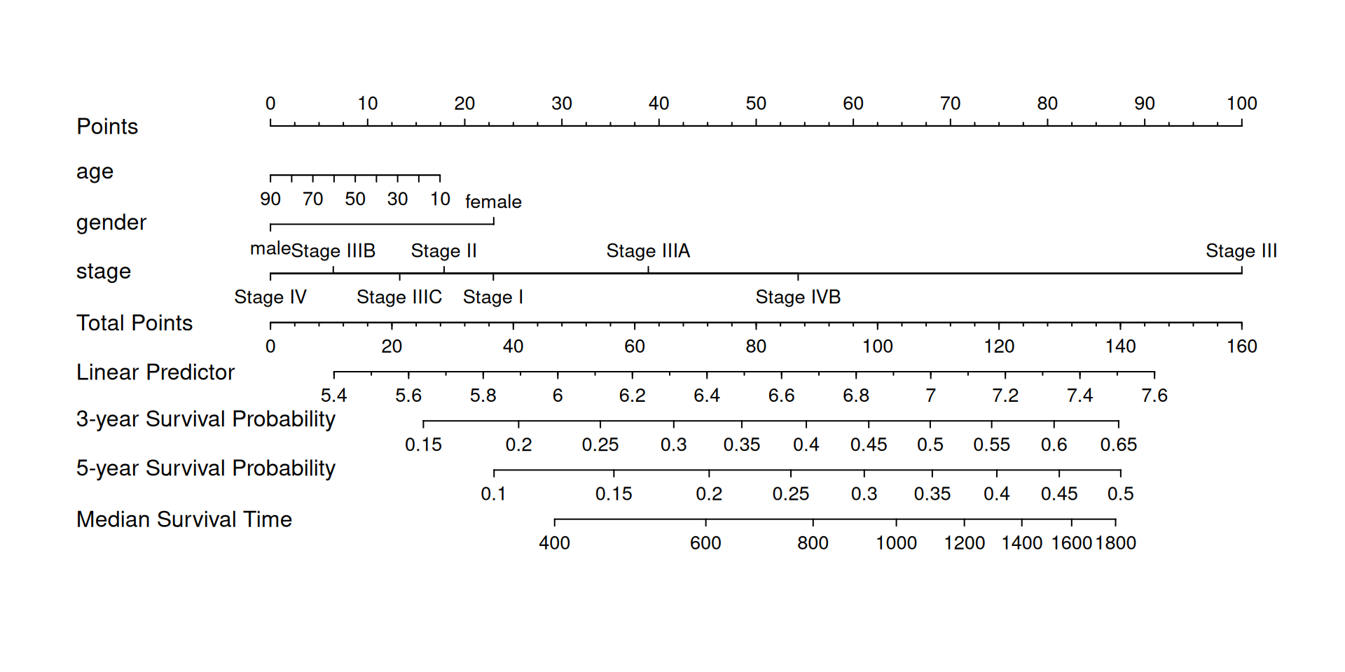

Figure 3: Predict 3-5 year survival probability

2. Beautify Nomogram

In addition to using nomogram for modeling and drawing, we can also use the survival package and regplot package for modeling and drawing. The figure below shows the construction and drawing of the model using a generalized linear model.

# Displays logistic regression, supports "lm", "glm", "coxph", "survreg" and "negbin"
## Plot a logistic regression, showing odds scale and confidence interval
lihcglm <- glm(status ~ age + gender + stage, data=LIHC )
regplot(lihcglm, 
        observation=LIHC[1,], 
        odds=TRUE, 
        interval="confidence")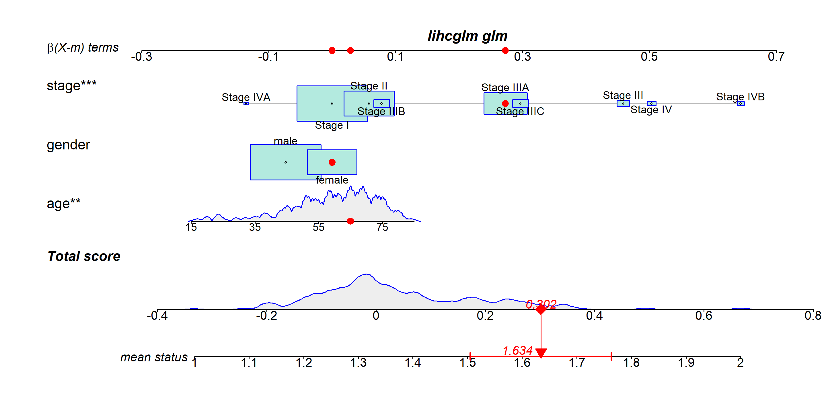

[1] "note: points tables not constructed unless points=TRUE "

The figure below shows the construction and drawing of the model using the generalized linear model.

lihccox <- coxph(formula = Surv(time,status) ~ age+gender+stage , data = LIHC)
regplot(lihccox,
        observation=LIHC[2,], # Scoring and displaying the indicators of observation 2 on the nomogram
        failtime = c(1095,1825),# Predict 3-year and 5-year mortality risk, the unit here is day
        prfail = TRUE, # TRUE is required in cox regression
        showP = T, # Whether statistical differences are shown
        droplines = F, # Observation 2 Example Scoring Whether to Draw a Line
        interval="confidence") # Displaying credible intervals for observations

[1] "note: points tables not constructed unless points=TRUE "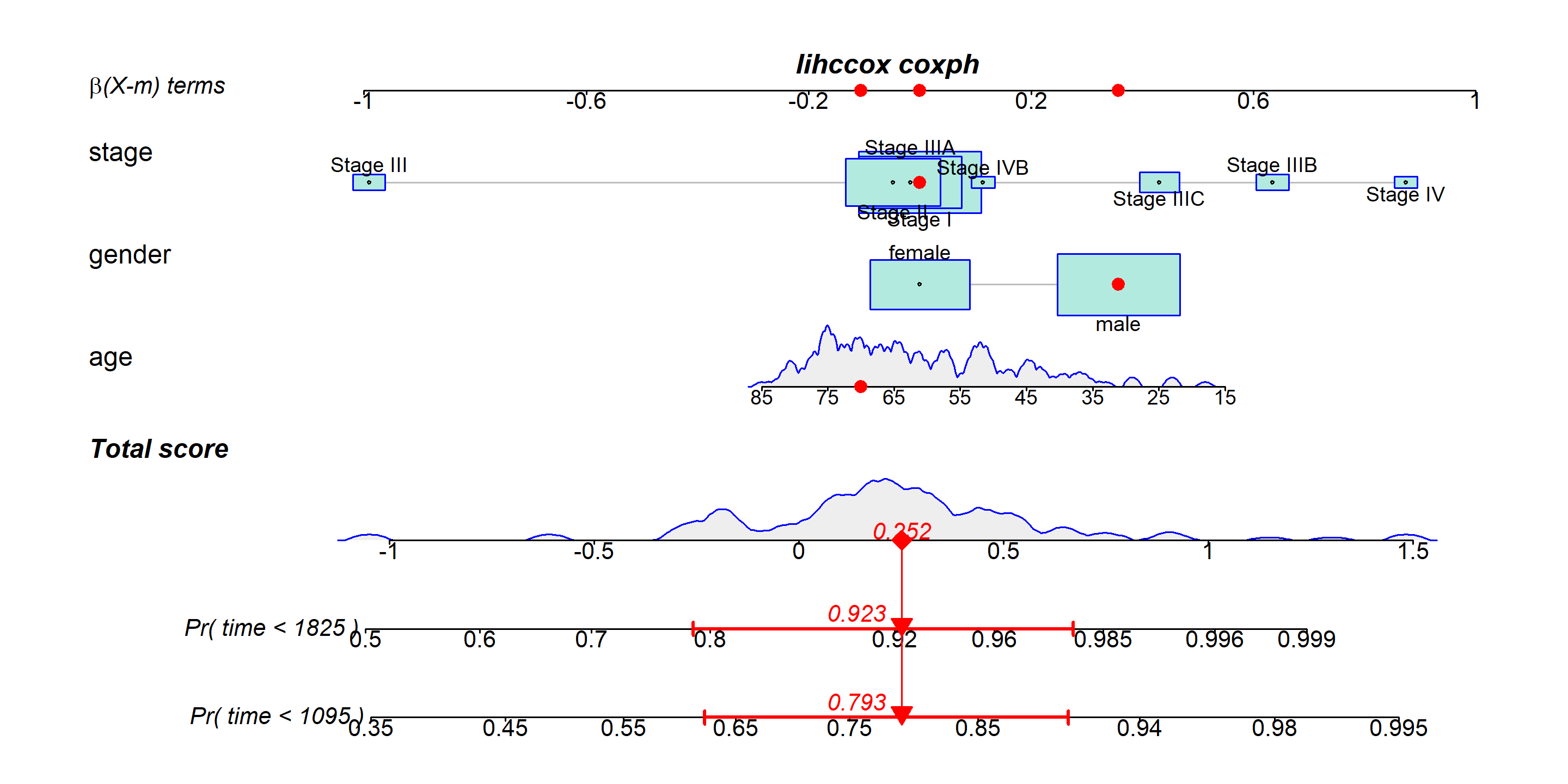

Application

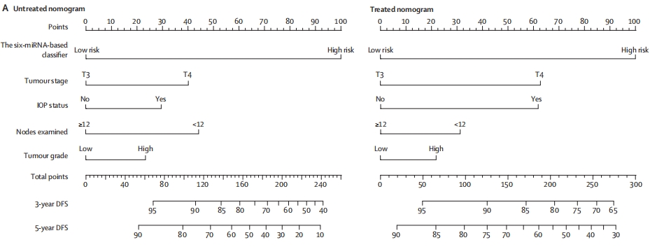
NomogramApp1 — Figure 4: Applications of Nomogram

This figure shows two schematics of clinical applications that integrate a 6-miRNA-based classifier with four clinicopathological risk factors to predict which patients are likely to benefit from adjuvant chemotherapy after surgery for stage II colon cancer. [2]

Reference

[1] Goldman MJ, Craft B, Hastie M, et al. Visualizing and interpreting cancer genomics data via the Xena platform. Nat Biotechnol. 2020;38(6):675-678. doi:10.1038/s41587-020-0546-8

[2] Zhang JX, Song W, Chen ZH, et al. Prognostic and predictive value of a microRNA signature in stage II colon cancer: a microRNA expression analysis [published correction appears in Lancet Oncol. 2014 Jan;15(1):e4]. Lancet Oncol. 2013;14(13):1295-1306. doi:10.1016/S1470-2045(13)70491-1