# 安装必要的包
if (!requireNamespace("ggplot2", quietly = TRUE)) {
  install.packages("ggplot2")
}
if (!requireNamespace("dplyr", quietly = TRUE)) {
  install.packages("dplyr")
}
if (!requireNamespace("tidyr", quietly = TRUE)) {
  install.packages("tidyr")
}
if (!requireNamespace("corrplot", quietly = TRUE)) {
  install.packages("corrplot")
}
if (!requireNamespace("ComplexHeatmap", quietly = TRUE)) {
  BiocManager::install("ComplexHeatmap")
}

# 加载包
library(ggplot2)
library(dplyr)
library(tidyr)
library(corrplot)
library(ComplexHeatmap)免疫亚型图
按免疫浸润 signature 评分对肿瘤样本聚类,正是泛癌免疫亚型(C1–C6)的定义方式 [1]:signature 评分两两求相关、把共变模块框出,再用评分把样本聚成亚型,各亚型的评分分布即其特征。本教程在模拟数据上复现这一版式:模块化的相关热图、样本聚成亚型、以及支撑命名的各亚型评分分布。
Example
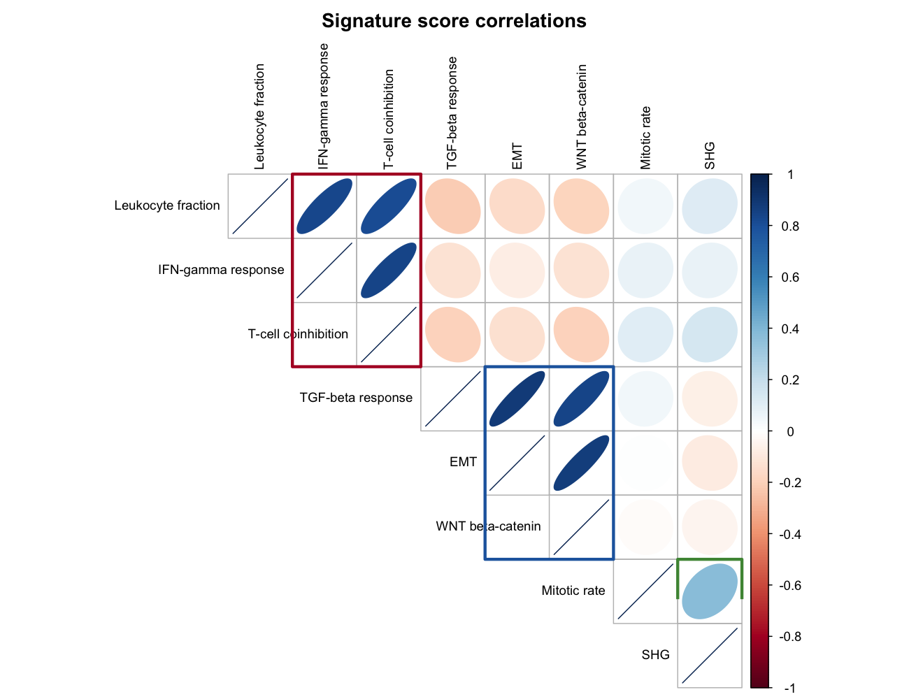
Setup
系统要求:跨平台(Linux/MacOS/Windows)
编程语言:R
依赖包:
ggplot2;dplyr;tidyr;corrplot;ComplexHeatmap
sessioninfo::session_info("attached")─ Session info ───────────────────────────────────────────────────────────────
setting value
version R version 4.6.2 (2026-10-29)
os Ubuntu 26.04.1 LTS
system x86_64, linux-gnu
ui X11
language (EN)
collate C.UTF-8
ctype C.UTF-8
tz UTC
date 2026-11-05
pandoc 3.7.0.2 @ /usr/bin/ (via rmarkdown)
quarto 1.11.9 @ /usr/local/bin/quarto
─ Packages ───────────────────────────────────────────────────────────────────
! package * version date (UTC) lib source
P ComplexHeatmap * 2.28.0 2026-04-28 [?] Bioconductor 3.23 (R 4.6.2)
P corrplot * 0.95 2024-10-14 [?] RSPM
P dplyr * 1.2.1 2026-04-03 [?] RSPM
P ggplot2 * 4.0.3.9000 2026-11-03 [?] Github (tidyverse/ggplot2@b638d65)
P tidyr * 1.3.2 2025-12-19 [?] RSPM
[1] /home/runner/.cache/R/renv/library/Bizard-5140bdc6/linux-ubuntu-resolute/R-4.6/x86_64-pc-linux-gnu
[2] /home/runner/work/_temp/Library
[3] /opt/R/4.6.2/lib/R/library
* ── Packages attached to the search path.
P ── Loaded and on-disk path mismatch.
──────────────────────────────────────────────────────────────────────────────Data Preparation
模拟 90 个样本 × 8 个免疫 signature 的评分,植入三个相关模块(白细胞/IFN-γ/T 细胞同高;EMT/WNT 同高且与前者相反;有丝分裂独立)——这正是产生清晰免疫亚型的结构。
set.seed(601)
signatures <- c("Leukocyte fraction", "IFN-gamma response", "T-cell coinhibition",
                "TGF-beta response", "EMT", "WNT beta-catenin", "Mitotic rate", "SHG")
n_sam <- 90
latent <- matrix(rnorm(n_sam * 3, sd = 1), nrow = n_sam)   # 3 个潜在因子

score_of <- function(factor_idx, coef, noise = 0.35) {
  as.numeric(latent[, factor_idx] %*% t(matrix(coef, 1)) + rnorm(n_sam, sd = noise))
}
sig_scores <- data.frame(
  sample = paste0("TCGA-", sprintf("%02d", 1:n_sam)),
  `Leukocyte fraction`  = score_of(1,  1.0),
  `IFN-gamma response`  = score_of(1,  0.9),
  `T-cell coinhibition` = score_of(1,  0.8),
  `TGF-beta response`   = score_of(2,  0.9),
  EMT                   = score_of(2,  0.9),
  `WNT beta-catenin`    = score_of(2,  0.7),
  `Mitotic rate`        = score_of(3,  1.0),
  SHG                   = score_of(3,  0.2),
  check.names = FALSE)

sig_mat <- as.matrix(sig_scores[, -1])
rownames(sig_mat) <- sig_scores$sample
head(sig_scores[, 1:4])
sample Leukocyte fraction IFN-gamma response T-cell coinhibition
1 TCGA-01 0.1246969 0.1222007 -0.4844777
2 TCGA-02 1.5600376 2.0504853 1.0776181
3 TCGA-03 -0.6165379 -0.3190881 0.1236476
4 TCGA-04 -0.1197363 0.1009733 -0.2371480
5 TCGA-05 -0.3245752 -0.2817904 -0.3067847
6 TCGA-06 -2.4798910 -1.3339186 -1.1086733Visualization
1. Signature 相关模块
cor_mat <- cor(sig_mat)
module <- c(1, 1, 1, 2, 2, 2, 3, 3)
mod_pal <- c("#B2182B", "#2166AC", "#4D9342")

corrplot(cor_mat, method = "ellipse", type = "upper",
         tl.col = "black", tl.cex = 0.8, col.lim = c(-1, 1),
         mar = c(0, 0, 2, 0),
         title = "Signature score correlations")
## corrplot upper-triangle grid: cell (i, j) sits at x = j, y = 9 - i
for (k in seq_len(3)) {
  idx <- which(module == k)
  rect(min(idx) + 0.5, 9 - max(idx) - 0.5,
       max(idx) + 0.5, 9 - min(idx) + 0.5,
       border = mod_pal[k], lwd = 3, lend = 1)
}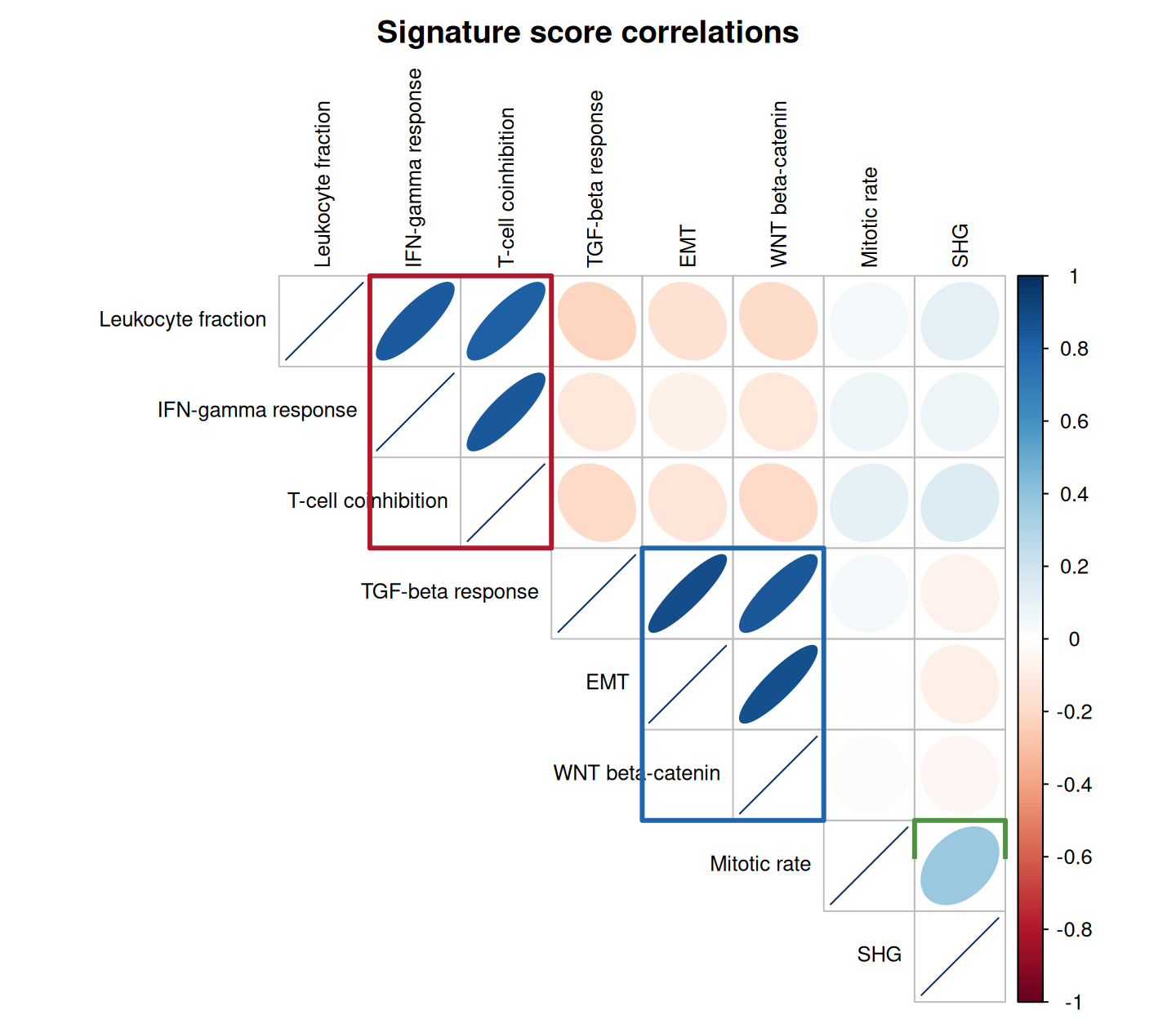
三个矩形把 signature 分成共变模块——即参考论文在共识聚类周围框出的结构。
2. 样本聚成免疫亚型
## 参考流程用 ConsensusClusterPlus;z-score 矩阵的层次聚类是免依赖替代
z_mat <- t(scale(sig_mat))     # signature x 样本,按 signature 标准化
hcs <- hclust(dist(t(z_mat)), method = "ward.D2")
n_sub <- 6
subtype <- paste0("C", cutree(hcs, k = n_sub))

col_fun <- circlize::colorRamp2(c(-2, 0, 2), c("#2166AC", "white", "#B2182B"))
ha <- HeatmapAnnotation(Subtype = subtype,
                        col = list(Subtype = c("C1" = "#F2CCCC", "C2" = "#B31E22",
                                               "C3" = "#529B40", "C4" = "#020105",
                                               "C5" = "#383D8E", "C6" = "#EABF00")),
                        show_legend = FALSE)
Heatmap(z_mat, name = "Score (z)", top_annotation = ha,
        col = col_fun, cluster_columns = hcs,
        show_column_names = FALSE,
        row_names_gp = grid::gpar(fontsize = 8),
        column_split = 6,          # with a dendrogram, split takes k, not a factor
        column_gap = unit(1.5, "mm"),
        border = TRUE)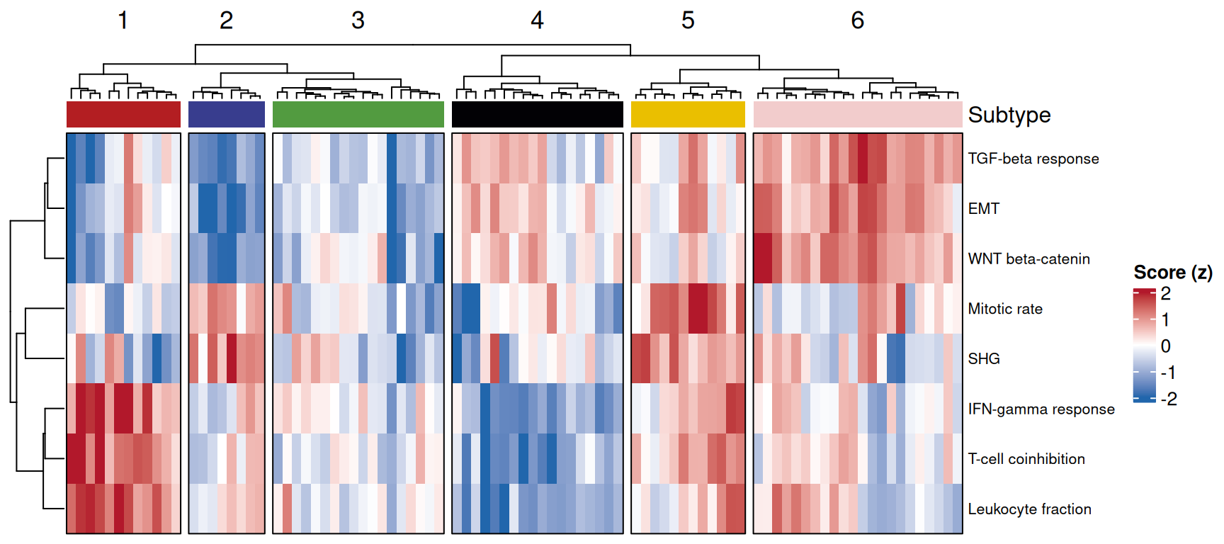
每个列分块是一个亚型;色块展示哪些 signature 占主导。真实数据的亚型判定请用作者后续写的 ImmuneSubtypeClassifier 包,比原始流程更稳健。
3. 各亚型的评分分布
show_sigs <- c("Leukocyte fraction", "TGF-beta response", "Mitotic rate")
dist_df <- sig_scores |>
  mutate(subtype = subtype) |>
  pivot_longer(all_of(show_sigs), names_to = "Signature", values_to = "Score")

ggplot(dist_df, aes(subtype, Score, fill = subtype)) +
  geom_boxplot(outlier.shape = NA, width = 0.65) +
  geom_hline(yintercept = 0, linetype = "dashed", colour = "grey40") +
  facet_wrap(~Signature, nrow = 1) +
  scale_fill_manual(values = c("C1" = "#F2CCCC", "C2" = "#B31E22", "C3" = "#529B40",
                               "C4" = "#020105", "C5" = "#383D8E", "C6" = "#EABF00")) +
  labs(x = NULL, y = "Signature score", fill = "Subtype") +
  theme_classic(base_size = 11) +
  theme(legend.position = "top", legend.key.size = unit(3, "mm"))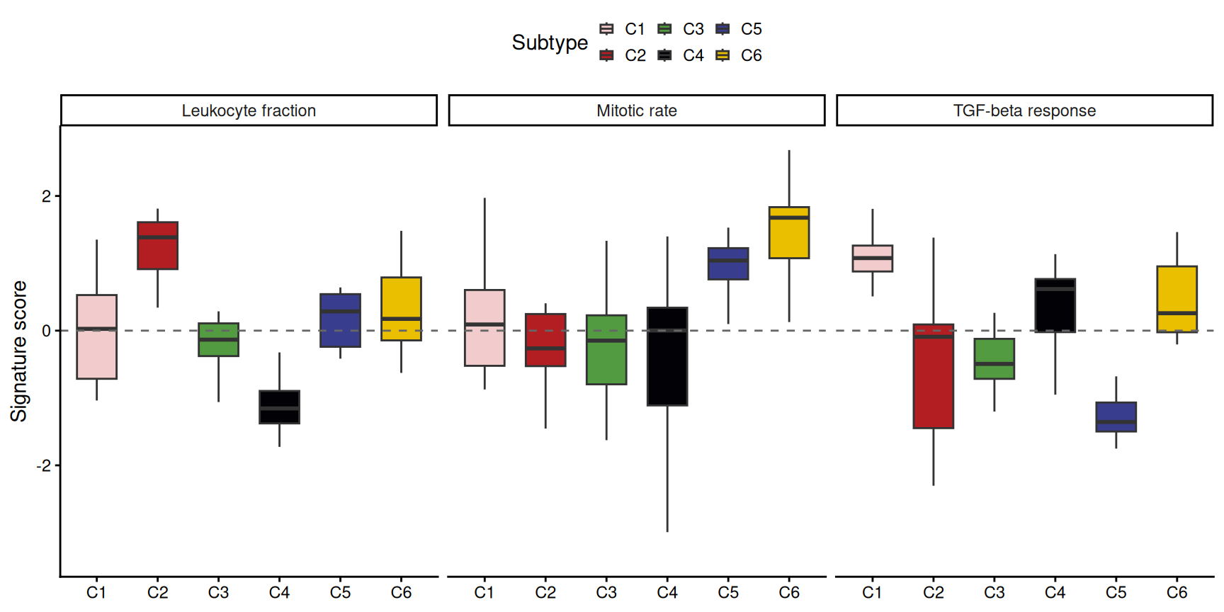
提示
实践要点
- 参考流程对基因定量方法非常敏感——FPKM/RPKM/TPM 上效果不佳;真实数据请用作者的
ImmuneSubtypeClassifier。 - 亚型按主导模块命名(如 C2 = IFN-γ 主导、C6 = TGF-β 主导);模拟数据可通过箱线面板目视命名。
- 模块热图与亚型分块放在同一张图:审稿人要核对聚类的模块正是亚型间有差异的那些。
Application
免疫亚型判定是免疫肿瘤队列的标准第一步注释:先分组再做 checkpoint 响应或 TMB 比较。上述版式(模块热图 → 亚型条带 → 评分分布)正是参考图报告它们的方式。
Reference
[1] Thorsson V, Gibbs DL, Brown SD, et al. The immune landscape of cancer. Immunity. 2018;48(4):812-830.e24. doi:10.1016/j.immuni.2018.03.023
[2] Xiaofan Lu, et al. FigureYa: A Standardized Visualization Framework for Enhancing Biomedical Data Interpretation and Research Efficiency. iMetaMed. 2025. doi:10.1002/imm3.70005