森林图（Python）

🤖 AI Skill — Download the Bizard unified skill for your AI assistant ⬇️ Download Skill ZIP

🔌 MCP Server — Let AI agents (Claude Code, Cursor, …) query Bizard live: claude mcp add bizard -- npx @openbiox/bizard-mcp — or the free hosted instance (no install, faster from mainland China): claude mcp add --transport http bizard http://biotree.top:38123/bizard-mcp/mcp 📖 MCP Docs

📖 Cite Bizard — if Bizard helps your research, please cite: Li, K., Zheng, H., Huang, K., et al. (2026). Bizard: A Community-Driven Platform for Accelerating and Enhancing Biomedical Data Visualization. iMetaMed, e70038. 🔗 DOI / BibTeX

森林图把每项研究的效应估计画成带置信区间的标记，标记大小随精度缩放，底部合并估计用菱形表达——这是 meta 分析和多预测变量回归表的标准展示。它由 matplotlib 的 hlines/scatter/Polygon 图元组装，对数刻度、无效线与权重等每个元素都清晰可控。

示例

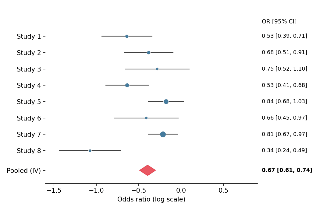
环境配置

• 系统要求：跨平台（Linux/MacOS/Windows）
• 编程语言：Python
• 依赖包：matplotlib、pandas、numpy

import matplotlib.pyplot as plt
from matplotlib.patches import Polygon
import pandas as pd
import numpy as np

数据准备

我们模拟一项二分类终点 meta 分析的八项研究：log 优势比围绕 −0.5 波动、研究特异标准误不同，并用逆方差法计算合并估计。

np.random.seed(151)

studies = pd.DataFrame({
    'Study': [f'Study {i}' for i in range(1, 9)],
    'logOR': np.random.normal(-0.5, 0.22, 8),
    'SE': np.random.uniform(0.08, 0.20, 8),
})
studies['CI_low'] = studies.logOR - 1.96 * studies.SE
studies['CI_high'] = studies.logOR + 1.96 * studies.SE
studies['Weight'] = 1 / studies.SE ** 2
pooled = pd.Series({
    'logOR': np.average(studies.logOR, weights=studies.Weight),
    'SE': np.sqrt(1 / studies.Weight.sum()),
})
pooled['CI_low'] = pooled.logOR - 1.96 * pooled.SE
pooled['CI_high'] = pooled.logOR + 1.96 * pooled.SE

可视化

带合并菱形的森林图

标记面积随逆方差权重缩放；无效线（OR = 1）与右侧效应值列构成完整的临床排版。

y = np.arange(len(studies))[::-1]

fig, ax = plt.subplots(figsize=(7, 4.6))
ax.hlines(y, studies.CI_low, studies.CI_high, color='0.25', linewidth=1.1)
ax.scatter(studies.logOR, y, s=studies.Weight * 90 / studies.Weight.max(),
           color='#457b9d', zorder=3, edgecolor='white', linewidth=0.5)
diamond_y = -1.2
diamond = Polygon([[pooled.CI_low, diamond_y], [pooled.logOR, diamond_y + 0.32],
                   [pooled.CI_high, diamond_y], [pooled.logOR, diamond_y - 0.32]],
                  closed=True, color='#e63946', alpha=0.85)
ax.add_patch(diamond)
ax.axvline(0, color='0.55', linewidth=0.9, linestyle='--')
ax.set_yticks(list(y) + [diamond_y], list(studies.Study) + ['Pooled (IV)'])
ax.text(1.02, y.max() + 0.9, 'OR [95% CI]', transform=ax.get_yaxis_transform(),
        fontsize=9, va='center')
ax.set_ylim(-2, len(studies) + 0.8)
for yi, (_, row) in zip(y, studies.iterrows()):
    ax.text(1.02, yi, f'{np.exp(row.logOR):.2f} '
            f'[{np.exp(row.CI_low):.2f}, {np.exp(row.CI_high):.2f}]',
            transform=ax.get_yaxis_transform(), fontsize=8.5, va='center')
ax.text(1.02, diamond_y, f'{np.exp(pooled.logOR):.2f} '
        f'[{np.exp(pooled.CI_low):.2f}, {np.exp(pooled.CI_high):.2f}]',
        transform=ax.get_yaxis_transform(), fontsize=8.5, va='center',
        fontweight='bold')
ax.set_xlabel('Odds ratio (log scale)')
ax.set_xlim(-1.6, 0.9)
ax.spines[['top', 'right', 'left']].set_visible(False)
plt.tight_layout()
plt.show()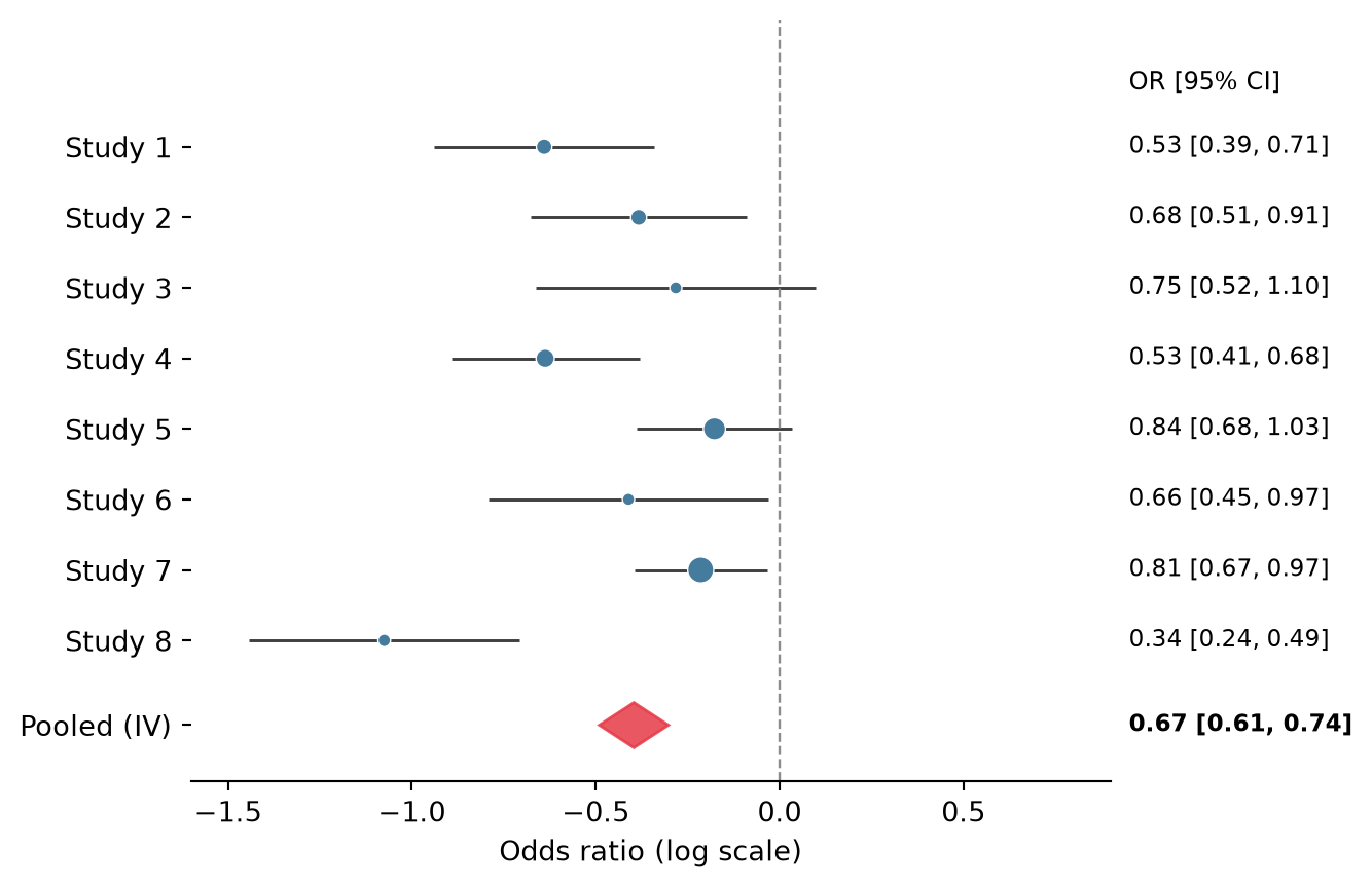

图 1: 含逆方差合并菱形的 meta 分析森林图

分亚组森林图

插入亚组标题并缩进其研究，可在不增加图形的情况下组织异质性证据。

studies['Subgroup'] = ['Retrospective'] * 4 + ['Prospective'] * 4

fig, ax = plt.subplots(figsize=(7, 5))
row = 0
yticks, ylabels = [], []
for subgroup, sub in studies.groupby('Subgroup', sort=False):
    ax.text(0, row, subgroup, fontsize=10, fontweight='bold', va='center')
    yticks.append(row); ylabels.append('')
    row -= 1
    for _, s in sub.iterrows():
        lo, hi = s.CI_low, s.CI_high
        ax.hlines(row, lo, hi, color='0.25', linewidth=1.1)
        ax.scatter(s.logOR, row, s=70, color='#457b9d',
                   zorder=3, edgecolor='white', linewidth=0.5)
        ax.text(1.02, row, f'{np.exp(s.logOR):.2f} '
                f'[{np.exp(lo):.2f}, {np.exp(hi):.2f}]',
                transform=ax.get_yaxis_transform(), fontsize=8.5, va='center')
        yticks.append(row); ylabels.append(s.Study)
        row -= 1
    row -= 0.6

diamond = Polygon([[pooled.CI_low, row], [pooled.logOR, row + 0.3],
                   [pooled.CI_high, row], [pooled.logOR, row - 0.3]],
                  closed=True, color='#e63946', alpha=0.85)
ax.add_patch(diamond)
ax.text(0, row, 'Pooled (IV)', fontsize=10, fontweight='bold', va='center')
ax.text(1.02, row, f'{np.exp(pooled.logOR):.2f} '
        f'[{np.exp(pooled.CI_low):.2f}, {np.exp(pooled.CI_high):.2f}]',
        transform=ax.get_yaxis_transform(), fontsize=8.5, va='center',
        fontweight='bold')
yticks.append(row); ylabels.append('')
ax.axvline(0, color='0.55', linewidth=0.9, linestyle='--')
ax.set_yticks(yticks, ylabels)
ax.set_xlabel('Odds ratio (log scale)')
ax.set_xlim(-1.6, 0.9)
ax.spines[['top', 'right', 'left']].set_visible(False)
plt.tight_layout()
plt.show()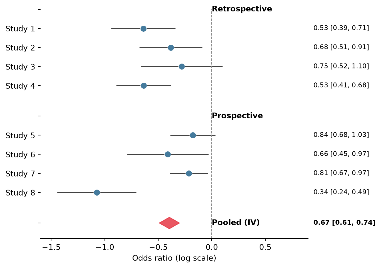

图 2: 带亚组标题的森林图

参考文献

1. Bax, L., Yu, L. M., Ikeda, N., Tsuruta, H., & Moons, K. G. (2006). Development and validation of MIX: comprehensive free software for meta-analysis of causal research data. BMC Medical Research Methodology, 6, 50.
2. Hunter, J. D. (2007). Matplotlib: A 2D graphics environment. Computing in Science & Engineering, 9(3), 90-95.