折线图（Python）

🤖 AI Skill — Download the Bizard unified skill for your AI assistant ⬇️ Download Skill ZIP

🔌 MCP Server — Let AI agents (Claude Code, Cursor, …) query Bizard live: claude mcp add bizard -- npx @openbiox/bizard-mcp — or the free hosted instance (no install, faster from mainland China): claude mcp add --transport http bizard http://biotree.top:38123/bizard-mcp/mcp 📖 MCP Docs

📖 Cite Bizard — if Bizard helps your research, please cite: Li, K., Zheng, H., Huang, K., et al. (2026). Bizard: A Community-Driven Platform for Accelerating and Enhancing Biomedical Data Visualization. iMetaMed, e70038. 🔗 DOI / BibTeX

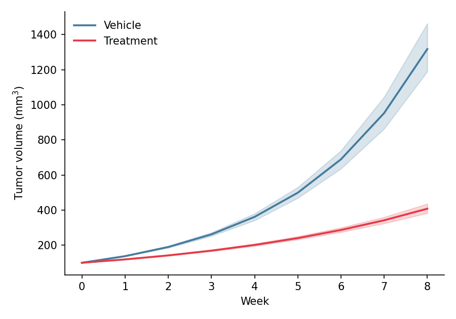
折线图展示连续变量沿有序轴（通常是时间）的趋势。在生物医学研究中，折线图是生长曲线、药代动力学轮廓和纵向组学时间序列的标准图形，通常在组均值周围附上不确定性带。Python 的 seaborn 只需一次调用即可将重复测量聚合为均值线与置信带，matplotlib 则提供更精细的样式控制。

示例

环境配置

• 系统要求：跨平台（Linux/MacOS/Windows）
• 编程语言：Python
• 依赖包：matplotlib、seaborn、pandas、numpy

import matplotlib.pyplot as plt
import seaborn as sns
import pandas as pd
import numpy as np

数据准备

我们模拟一项临床前肿瘤生长实验：两个处理臂（Vehicle 与 Treatment）各 12 只小鼠，连续 8 周每周测量一次，采用带小鼠间变异的两相指数生长模型。

np.random.seed(21)

weeks = np.arange(0, 9)
n_mice = 12
records = []
for arm, growth_rate in [('Vehicle', 0.32), ('Treatment', 0.18)]:
    for mouse in range(n_mice):
        size = 100 * np.exp(growth_rate * np.random.normal(1, 0.08) * weeks)
        records.append(pd.DataFrame({
            'Week': weeks,
            'Size': size,
            'Arm': arm,
            'Mouse': f'{arm[:2]}_{mouse:02d}'
        }))
tumor = pd.concat(records, ignore_index=True)

可视化

基础折线图

先聚合再绘图：每组一条线并配以不同 marker，使小型汇总图保持易读。

mean_size = tumor.groupby(['Arm', 'Week'], as_index=False)['Size'].mean()

plt.figure(figsize=(6, 4.2))
ax = sns.lineplot(data=mean_size, x='Week', y='Size', hue='Arm',
                  style='Arm', markers=['o', 's'], markersize=6,
                  palette={'Vehicle': '#457b9d', 'Treatment': '#e63946'},
                  linewidth=1.8)
ax.set_xlabel('Week')
ax.set_ylabel('Tumor volume (mm$^3$)')
ax.legend(frameon=False, title=None)
ax.spines[['top', 'right']].set_visible(False)
plt.tight_layout()
plt.show()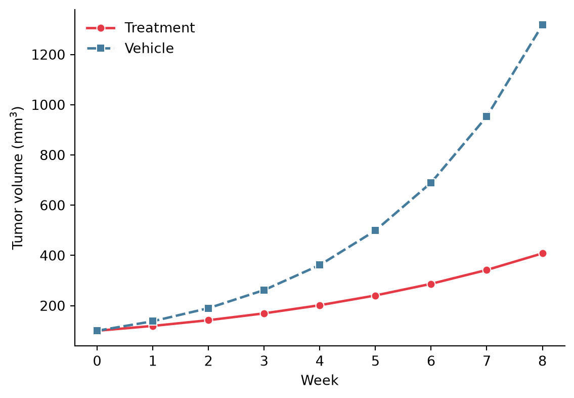

图 1: 两个处理臂每周的平均肿瘤体积

带置信带的折线图

将原始重复测量传入 seaborn.lineplot 并设置 errorbar=('ci', 95)，即可对每组均值进行自助法 95% 置信带估计——临床前研究图形的默认不确定性展示。

plt.figure(figsize=(6, 4.2))
ax = sns.lineplot(data=tumor, x='Week', y='Size', hue='Arm',
                  errorbar=('ci', 95), err_kws=dict(alpha=0.2),
                  palette={'Vehicle': '#457b9d', 'Treatment': '#e63946'},
                  linewidth=1.8)
ax.set_xlabel('Week')
ax.set_ylabel('Tumor volume (mm$^3$)')
ax.legend(frameon=False, title=None)
ax.spines[['top', 'right']].set_visible(False)
plt.tight_layout()
plt.show()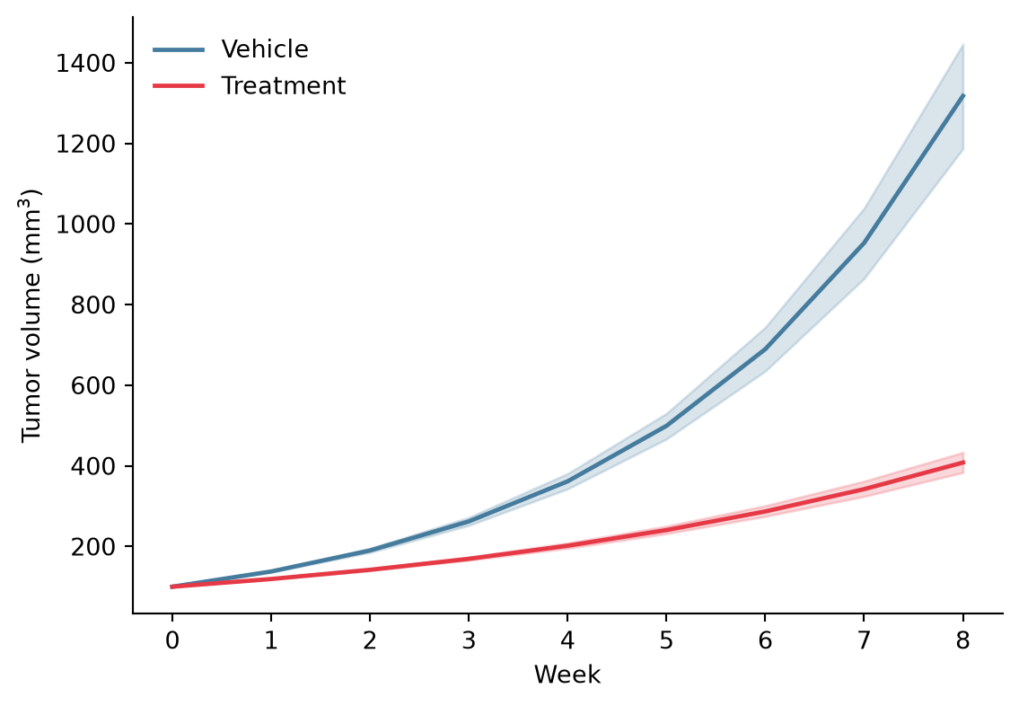

图 2: 组均值及自助法 95% 置信带

意大利面条图叠加群体均值

将每个受试对象画为细线并置于加粗组均值之后，同时传达趋势与个体间变异——许多期刊比单纯置信带更青睐这种形式。

fig, ax = plt.subplots(figsize=(6, 4.2))
sns.lineplot(data=tumor, x='Week', y='Size', hue='Arm', units='Mouse',
             estimator=None, alpha=0.25, linewidth=0.9, legend=False,
             palette={'Vehicle': '#457b9d', 'Treatment': '#e63946'}, ax=ax)
mean_size = tumor.groupby(['Arm', 'Week'], as_index=False)['Size'].mean()
sns.lineplot(data=mean_size, x='Week', y='Size', hue='Arm',
             palette={'Vehicle': '#457b9d', 'Treatment': '#e63946'},
             linewidth=2.4, ax=ax)
ax.set_xlabel('Week')
ax.set_ylabel('Tumor volume (mm$^3$)')
ax.legend(frameon=False, title=None)
ax.spines[['top', 'right']].set_visible(False)
plt.tight_layout()
plt.show()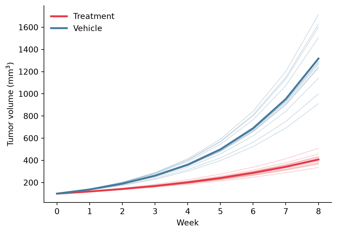

图 3: 个体生长曲线（细线）与组均值（粗线）

参考文献

1. Hunter, J. D. (2007). Matplotlib: A 2D graphics environment. Computing in Science & Engineering, 9(3), 90-95.
2. Waskom, M. L. (2021). seaborn: statistical data visualization. Journal of Open Source Software, 6(60), 3021.