GSEA 运行得分图

作者

[贡献] ZCode (GLM) — AI 生成，独立 AI 复核

修改于

2026-10-31

🤖 AI Skill — Download the Bizard unified skill for your AI assistant ⬇️ Download Skill ZIP

🔌 MCP Server — Let AI agents (Claude Code, Cursor, …) query Bizard live: claude mcp add bizard -- npx @openbiox/bizard-mcp — or the free hosted instance (no install, faster from mainland China): claude mcp add --transport http bizard http://biotree.top:38123/bizard-mcp/mcp 📖 MCP Docs

📖 Cite Bizard — if Bizard helps your research, please cite: Li, K., Zheng, H., Huang, K., et al. (2026). Bizard: A Community-Driven Platform for Accelerating and Enhancing Biomedical Data Visualization. iMetaMed, e70038. 🔗 DOI / BibTeX

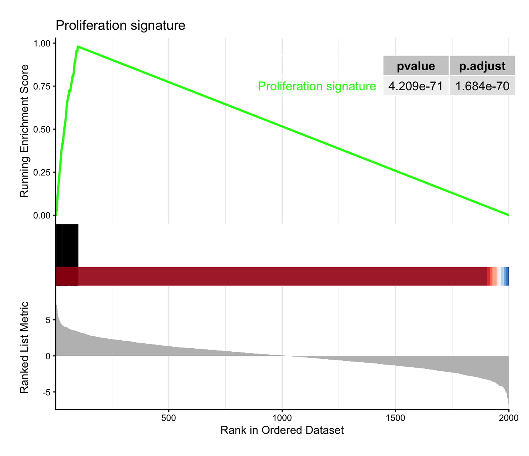
基因集富集分析（GSEA）检验一个已定义的基因集（通路、特征基因）是否在全基因组排序表中聚集在一端 [1]。它的经典配图是运行得分图：排序统计量以条形码形式展示（顶部），行走的富集得分在基因集成员命中处上升、在未命中处下降，峰值即富集得分（中部），基因集成员位置以毯子图（rug）标出（底部）。与过表达分析不同，GSEA 使用完整排序表——不需要对输入基因人为设定显著性截断——这正是”图”而非”表”承载论证的原因。

在 R 中分析由 clusterProfiler::GSEA() [2] 完成，经典图形由 enrichplot::gseaplot2() [3] 绘制。本教程绘制经典图形、在同一排序表上叠加多个基因集，并用 ggplot2 从基本组件重建运行得分，使统计量本身变得可读。本教程的 Python 对应版本见 GSEA 运行得分图（Python）。

本教程涵盖三种工作流：

经典 gseaplot2 运行得分图（带 p 值表）；
多个基因集叠加在同一排序表上；
手绘三面板运行 ES 重建（ggplot2 + patchwork）。

Example

Setup

系统要求：跨平台（Linux/MacOS/Windows）
编程语言：R
依赖包：clusterProfiler；enrichplot；ggplot2；dplyr；patchwork

# 安装必要的包（Bioconductor）
if (!requireNamespace("BiocManager", quietly = TRUE)) {
  install.packages("BiocManager")
}
if (!requireNamespace("clusterProfiler", quietly = TRUE)) {
  BiocManager::install("clusterProfiler")
}
if (!requireNamespace("patchwork", quietly = TRUE)) {
  install.packages("patchwork")
}

# 加载包
library(clusterProfiler)
library(enrichplot)
library(ggplot2)
library(dplyr)
library(patchwork)

sessioninfo::session_info("attached")

─ Session info ───────────────────────────────────────────────────────────────
 setting  value
 version  R version 4.6.2 (2026-10-29)
 os       Ubuntu 24.04.5 LTS
 system   x86_64, linux-gnu
 ui       X11
 language (EN)
 collate  C.UTF-8
 ctype    C.UTF-8
 tz       UTC
 date     2026-10-30
 pandoc   3.1.3 @ /usr/bin/ (via rmarkdown)
 quarto   1.10.19 @ /usr/local/bin/quarto

─ Packages ───────────────────────────────────────────────────────────────────
 ! package         * version    date (UTC) lib source
 P clusterProfiler * 4.20.3     2026-10-19 [?] Bioconductor 3.23 (R 4.6.2)
 P dplyr           * 1.2.1      2026-04-03 [?] RSPM
 P enrichplot      * 1.32.1     2026-09-28 [?] Bioconductor 3.23 (R 4.6.2)
 P ggplot2         * 4.0.3.9000 2026-10-30 [?] Github (tidyverse/ggplot2@b638d65)
 P patchwork       * 1.3.2      2025-08-25 [?] RSPM

 [1] /home/runner/.cache/R/renv/library/Bizard-5140bdc6/linux-ubuntu-noble/R-4.6/x86_64-pc-linux-gnu
 [2] /home/runner/work/_temp/Library
 [3] /opt/R/4.6.2/lib/R/library

 * ── Packages attached to the search path.
 P ── Loaded and on-disk path mismatch.

──────────────────────────────────────────────────────────────────────────────

Data Preparation

为保证教程完全可复现，我们模拟排序表与基因集而非下载 MSigDB：2,000 个基因按 Wald 式统计量排序；一个集中在排序顶部的 60 基因”增殖”集、一个位于底部的 50 基因”代谢”集，以及两个中性集——这一配置能产生干净可读的富集得分。clusterProfiler::GSEA() 需要”命名且降序排序”的数值向量（geneList）和 TERM2GENE 数据框。

set.seed(251)

n_genes <- 2000
genes <- paste0("Gene", sprintf("%04d", 1:n_genes))
stats <- rnorm(n_genes, sd = 2)
names(stats) <- genes

geneList <- sort(stats, decreasing = TRUE)   # 必须降序排序

# 模拟基因集：一个在顶部、一个在底部、两个中性
gs_up   <- sample(genes[order(stats, decreasing = TRUE)[1:100]], 60)
gs_down <- sample(genes[order(stats)[1:100]], 50)
gs_neu1 <- sample(genes, 80)
gs_neu2 <- sample(genes, 70)

term2gene <- dplyr::bind_rows(
  data.frame(term = "Proliferation signature",     gene = gs_up),
  data.frame(term = "Metabolic repression",        gene = gs_down),
  data.frame(term = "Hypoxia response",            gene = gs_neu1),
  data.frame(term = "Immune checkpoint pathway",   gene = gs_neu2)
)

set.seed(251)  # GSEA 对基因集做置换抽样；保持 p 值可复现
gser <- GSEA(geneList, TERM2GENE = term2gene,
             minGSSize = 40, maxGSSize = 500,
             pvalueCutoff = 1,      # 教学目的保留全部基因集
             eps = 0, seed = TRUE, verbose = FALSE)

as.data.frame(gser) |>
  dplyr::select(ID, setSize, enrichmentScore, NES, pvalue, p.adjust)

                                                 ID setSize enrichmentScore
Proliferation signature     Proliferation signature      60       0.9798969
Metabolic repression           Metabolic repression      50      -0.9743590
Hypoxia response                   Hypoxia response      80       0.2660821
Immune checkpoint pathway Immune checkpoint pathway      70      -0.2202139
                                NES       pvalue     p.adjust
Proliferation signature    3.951487 6.001589e-73 2.400636e-72
Metabolic repression      -3.780863 4.617454e-58 9.234909e-58
Hypoxia response           1.136434 2.030361e-01 2.707147e-01
Immune checkpoint pathway -0.925151 6.088710e-01 6.088710e-01

Metabolic repression 的负 NES 表示该基因集聚集在排序表底部（下调基因）；中性集的 NES 在 0 附近徘徊。

Visualization

1. 经典运行得分图

gseaplot2(gser, geneSetID = 1, pvalue_table = TRUE,
          title = "Proliferation signature")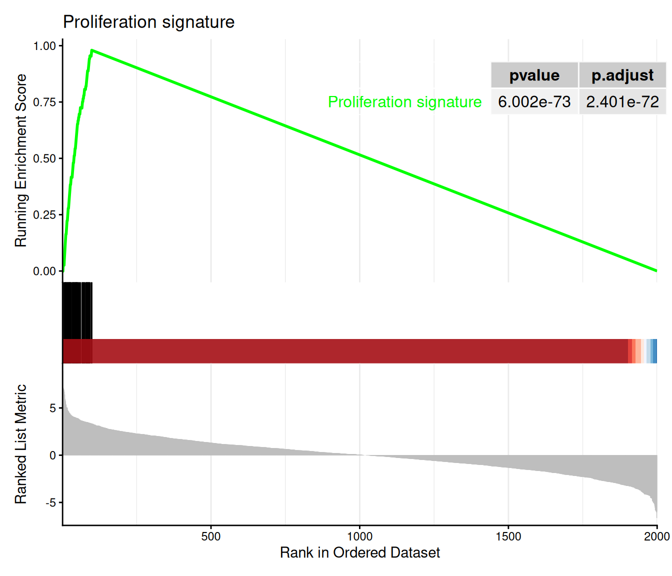

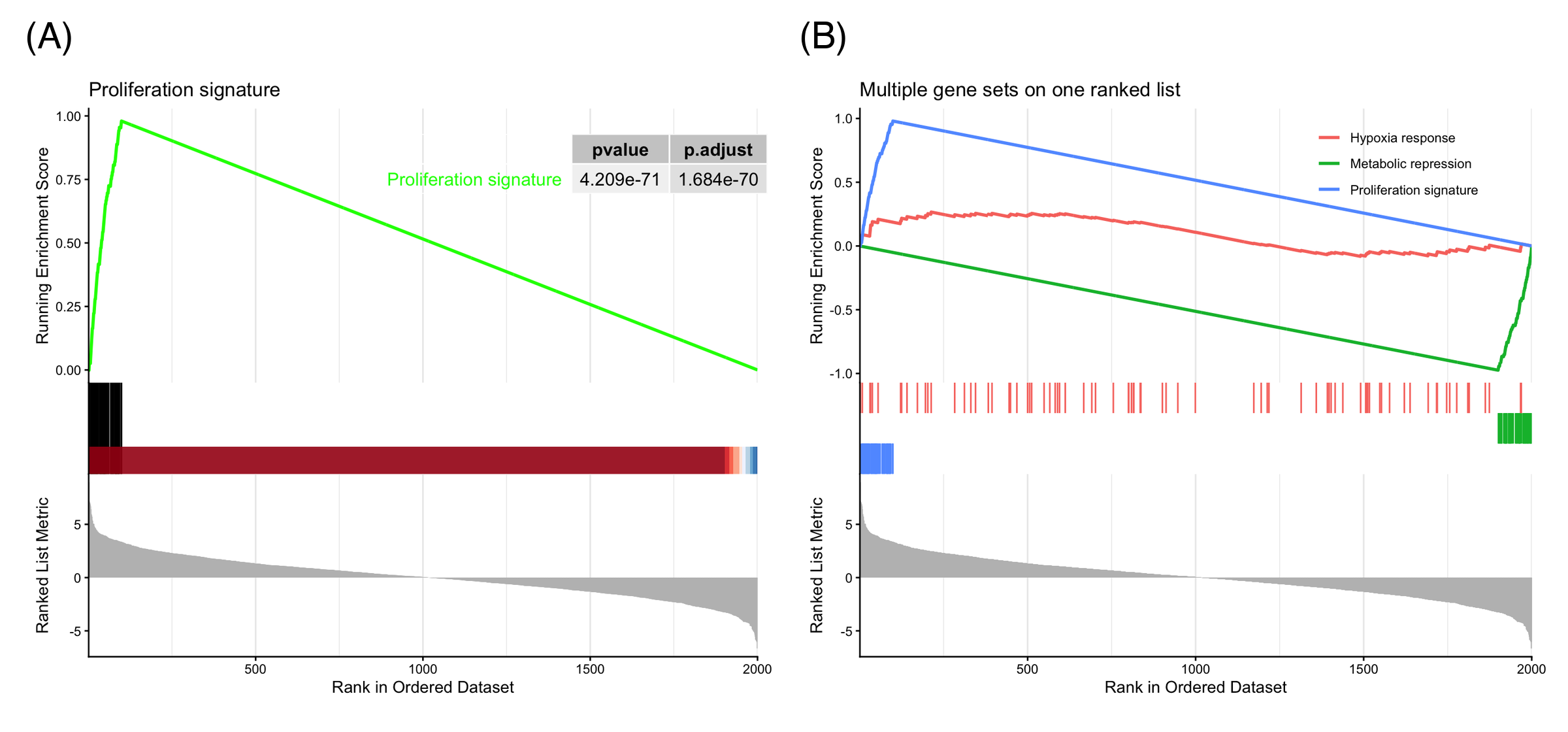
图 1: 顶部基因集的 gseaplot2：运行富集得分在 ES ≈ 0.98 处达峰、命中毯子图与排序统计量；插图报告置换 p 值。

三个面板共享同一横轴（排名位置）：运行 ES 在前 100 名（基因集成员所在）陡峭爬升、在富集得分处达峰后衰减；毯子图标出成员位置；底部曲线即排序统计量本身。峰值位置定义leading edge——驱动富集的基因。

2. 同一排序表上的多个基因集

ids <- match(c("Proliferation signature", "Metabolic repression", "Hypoxia response"),
             gser$ID)
gseaplot2(gser, geneSetID = ids, pvalue_table = FALSE,
          title = "Multiple gene sets on one ranked list")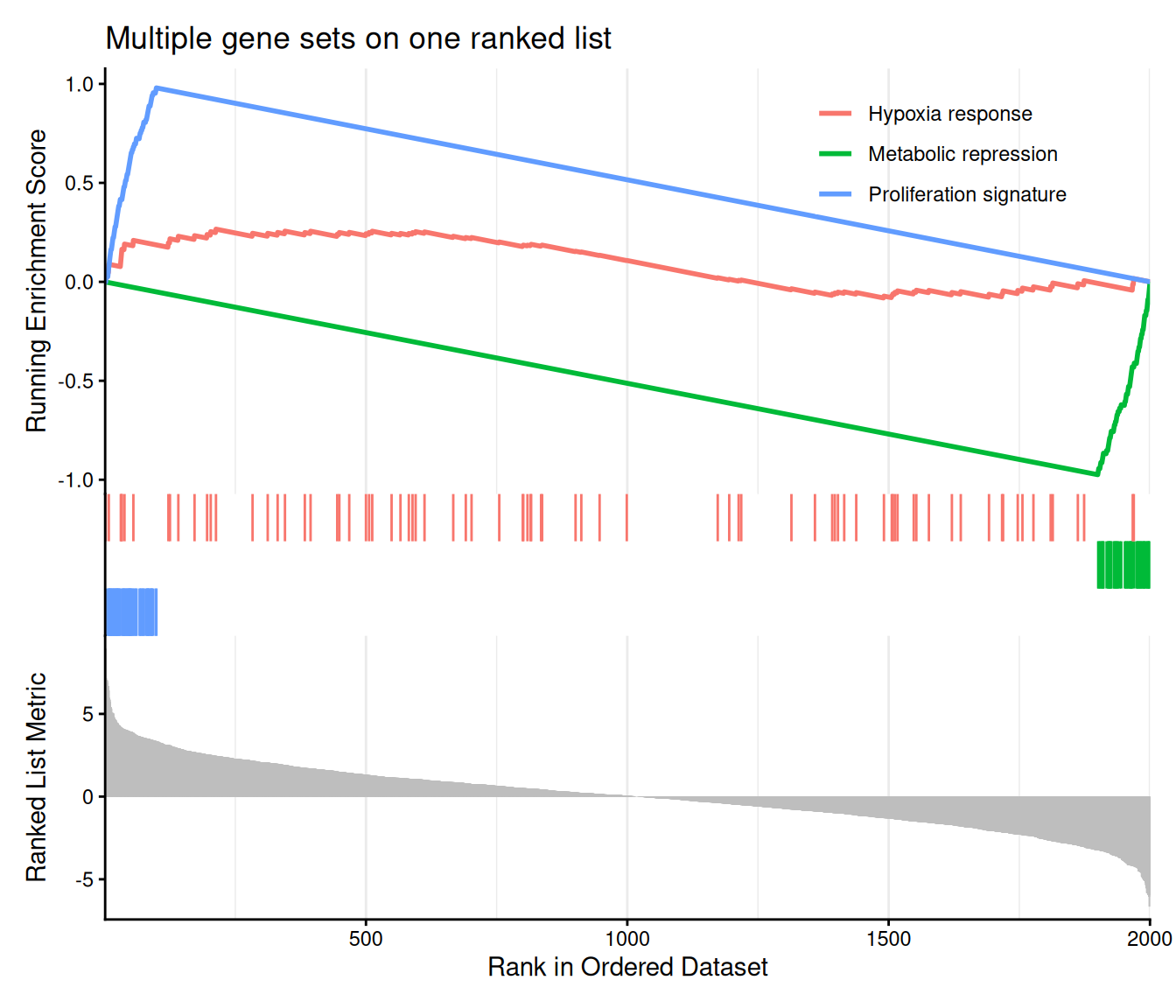

图 2: 同一排序表上叠加三个基因集：顶部富集集（NES 为正）、底部富集集（NES 为负）与中性集。

叠加基因集是比较 GSEA 结果的日常方式：上调富集的集早早达峰并缓慢衰减，下调富集的集在排序表末端俯冲至负的最小值，零假设下的集在 0 附近徘徊。图例标签跟随所选基因集；color 参数控制调色板。

3. 从基本组件重建运行得分

in_set  <- names(geneList) %in% gs_up
w       <- abs(geneList)
step    <- ifelse(in_set, w / sum(w[in_set]), -1 / sum(!in_set))
run_es  <- cumsum(step)
peak    <- which.max(run_es)

df <- data.frame(rank = seq_along(geneList),
                 stat = as.numeric(geneList),
                 es = run_es, hit = in_set)

p_top <- ggplot(df, aes(rank, stat)) +
  geom_segment(aes(xend = rank, yend = 0, color = hit),
               linewidth = 0.15, show.legend = FALSE) +
  scale_color_manual(values = c(`FALSE` = "grey70", `TRUE` = "#e63946")) +
  geom_vline(xintercept = peak, linetype = "dashed",
             color = "#1d3557", alpha = 0.5) +
  labs(y = "Ranked statistic", x = NULL) +
  theme_classic()

p_mid <- ggplot(df, aes(rank, es)) +
  geom_line(color = "#1d3557", linewidth = 0.8) +
  geom_point(data = df[peak, ], color = "#e63946", size = 2) +
  annotate("text", x = peak, y = max(run_es), vjust = -0.8, hjust = 0,
           label = sprintf("ES = %.2f at rank %d", max(run_es), peak), size = 3.5) +
  labs(y = "Running ES", x = NULL) +
  theme_classic()

p_rug <- ggplot(df[df$hit, ], aes(x = rank, y = 1)) +
  geom_segment(aes(xend = rank, yend = 0.55),
               linewidth = 0.3, color = "#e63946") +
  scale_y_continuous(limits = c(0, 1), expand = c(0, 0)) +
  theme_void()

p3 <- p_top / p_mid / p_rug +
  plot_layout(heights = c(3, 2, 0.5))
p3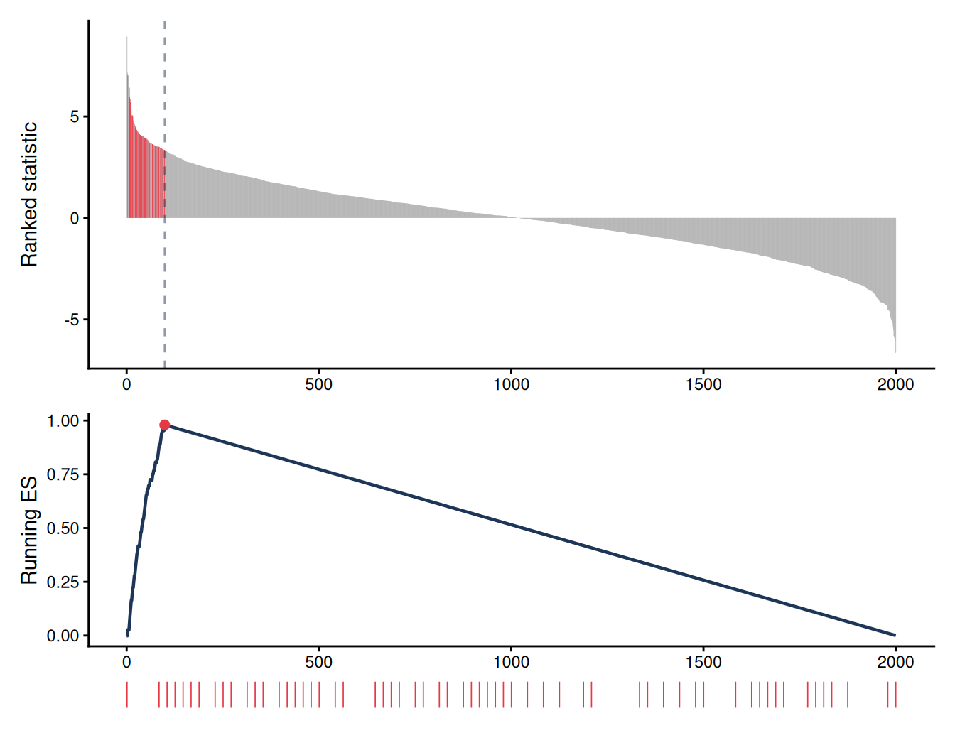

图 3: 手绘三面板运行得分图：加权 Kolmogorov-Smirnov 式统计量就是在成员处加正步长、在未命中处加负步长的累计和。

加权运行 ES 是一个累计和：在基因集成员处加上其 |统计量| 除以成员总权重，在未命中处减去 1/(N − n)。从基本组件重建它揭开了 gseaplot2 的面纱——第 1 节的曲线正是这条行走轨迹——也让自定义变体（leading edge 注释、分面板主题、多图版式）变得直观。

实践要点

geneList 必须是命名且降序排序的数值向量，否则 GSEA() 报错 “geneList should be a decreasing sorted vector”。
探索阶段用 pvalueCutoff = 1，避免被过滤的基因集从结果对象中悄悄消失。
传入 seed = TRUE（配合 set.seed()）保证置换 p 值可复现。
报告 NES 配合 p.adjust，而非原始 ES：ES 依赖基因集大小，NES 已对其标准化。

Application

运行得分 GSEA 图是转录组差异通路水平解读的标准配图：肿瘤-正常特征、药物扰动筛选和单细胞聚类标志基因。下图模拟典型论文版式：(A) 带p值表的经典单集图，(B) 多集叠加图。

Reference

[1] Subramanian A, Tamayo P, Mootha VK, et al. Gene set enrichment analysis: a knowledge-based approach for interpreting genome-wide expression profiles. Proc Natl Acad Sci USA. 2005;102(43):15545-15550. doi:10.1073/pnas.0506580102

[2] Wu T, Hu E, Xu S, et al. clusterProfiler 4.0: a universal enrichment tool for interpreting omics data. Innovation. 2021;2(3):100141. doi:10.1016/j.xinn.2021.100141

[3] Yu G. enrichplot: visualization of functional enrichment result. Bioconductor package. https://bioconductor.org/packages/enrichplot/