t-SNE 图

作者

[贡献] ZCode (GLM) — AI 生成，独立 AI 复核

修改于

2026-10-31

🤖 AI Skill — Download the Bizard unified skill for your AI assistant ⬇️ Download Skill ZIP

🔌 MCP Server — Let AI agents (Claude Code, Cursor, …) query Bizard live: claude mcp add bizard -- npx @openbiox/bizard-mcp — or the free hosted instance (no install, faster from mainland China): claude mcp add --transport http bizard http://biotree.top:38123/bizard-mcp/mcp 📖 MCP Docs

📖 Cite Bizard — if Bizard helps your research, please cite: Li, K., Zheng, H., Huang, K., et al. (2026). Bizard: A Community-Driven Platform for Accelerating and Enhancing Biomedical Data Visualization. iMetaMed, e70038. 🔗 DOI / BibTeX

t 分布随机邻域嵌入（t-SNE）把高维数据——每个细胞数千个基因、每个样本数百个特征——投影到保持”邻近观测相互靠近”的二维地图上 [1]。它是单细胞基因组学的主力嵌入方法：在两万个维度的表达空间中分离的细胞类型，在 t-SNE 平面上呈现为肉眼可见的”岛屿”，使群体结构一目了然。

t-SNE 回答的是结构问题（“有多少个群体、谁与谁相邻”），而不是距离问题：图上簇间距离与簇大小不具备全局含义，且图形随 perplexity 超参数和随机种子而变。PCA 保留全局几何但只能捕捉线性结构——两者互补，标准做法是在前若干个主成分上运行 t-SNE，而非直接在原始特征上 [2]。

本教程涵盖 Rtsne [3] 的四种实用工作流：

模拟单细胞表达矩阵的基础 t-SNE 地图；
perplexity 如何重塑图形（最需要检查的单一参数）；
同一数据上的 t-SNE 与 PCA 对比；
将标记基因表达叠加到地图上。

Example

Setup

系统要求：跨平台（Linux/MacOS/Windows）
编程语言：R
依赖包：Rtsne；ggplot2；dplyr；patchwork

# 安装必要的包
if (!requireNamespace("Rtsne", quietly = TRUE)) {
  install.packages("Rtsne")
}
if (!requireNamespace("patchwork", quietly = TRUE)) {
  install.packages("patchwork")
}

# 加载包
library(Rtsne)
library(ggplot2)
library(dplyr)
library(patchwork)

sessioninfo::session_info("attached")

─ Session info ───────────────────────────────────────────────────────────────
 setting  value
 version  R version 4.6.2 (2026-10-29)
 os       Ubuntu 24.04.5 LTS
 system   x86_64, linux-gnu
 ui       X11
 language (EN)
 collate  C.UTF-8
 ctype    C.UTF-8
 tz       UTC
 date     2026-10-31
 pandoc   3.1.3 @ /usr/bin/ (via rmarkdown)
 quarto   1.10.20 @ /usr/local/bin/quarto

─ Packages ───────────────────────────────────────────────────────────────────
 ! package   * version    date (UTC) lib source
 P dplyr     * 1.2.1      2026-04-03 [?] RSPM
 P ggplot2   * 4.0.3.9000 2026-10-30 [?] Github (tidyverse/ggplot2@b638d65)
 P patchwork * 1.3.2      2025-08-25 [?] RSPM
 P Rtsne     * 0.17       2023-12-07 [?] RSPM

 [1] /home/runner/.cache/R/renv/library/Bizard-5140bdc6/linux-ubuntu-noble/R-4.6/x86_64-pc-linux-gnu
 [2] /home/runner/work/_temp/Library
 [3] /opt/R/4.6.2/lib/R/library

 * ── Packages attached to the search path.
 P ── Loaded and on-disk path mismatch.

──────────────────────────────────────────────────────────────────────────────

Data Preparation

我们模拟类似 scRNA-seq 的对数表达矩阵：1,200 个细胞来自四个群体（CD4 T 细胞、B 细胞、NK 细胞、单核细胞）× 200 个基因，每个群体特异表达一段 20 基因的标记块。四个群体仅靠标记块区分——这正是 t-SNE 应当还原为四个岛屿的结构。

set.seed(251)

n_per   <- 300
types   <- c("CD4 T cells", "B cells", "NK cells", "Monocytes")
n_genes <- 200

base <- matrix(rnorm(n_per * length(types) * n_genes, 0, 0.6),
               nrow = n_per * length(types), ncol = n_genes,
               dimnames = list(NULL, paste0("Gene", 1:n_genes)))
ct <- rep(types, each = n_per)
markers <- list("CD4 T cells" = 1:20, "B cells" = 21:40,
                "NK cells" = 41:60, "Monocytes" = 61:80)
for (t in types) {
  idx <- which(ct == t)
  base[idx, markers[[t]]] <- base[idx, markers[[t]]] + 2.5
}
expr <- pmax(base + rnorm(length(base), 0, 0.3), 0)

# 标准做法：在前若干主成分上运行 t-SNE，而非原始基因
pcs <- prcomp(expr, rank. = 30)$x[, 1:30]

Visualization

1. 基础 t-SNE 地图

set.seed(251)                       # t-SNE 是随机算法：固定种子
tsne30 <- Rtsne(pcs, dims = 2, perplexity = 30, pca = FALSE, verbose = FALSE)

d30 <- data.frame(tSNE1 = tsne30$Y[, 1], tSNE2 = tsne30$Y[, 2], celltype = ct)
cent <- d30 |>
  group_by(celltype) |>
  summarise(tSNE1 = mean(tSNE1), tSNE2 = mean(tSNE2))

pal <- c("#4E79A7", "#F28E2B", "#E15759", "#76B7B2")
p1 <- ggplot(d30, aes(tSNE1, tSNE2, color = celltype)) +
  geom_point(size = 0.7, alpha = 0.8) +
  geom_text(data = cent, aes(tSNE1, tSNE2, label = celltype),
            inherit.aes = FALSE, color = "black",
            fontface = "bold", size = 3.5, vjust = -1.2) +
  scale_color_manual(values = pal) +
  labs(x = "t-SNE 1", y = "t-SNE 2") +
  theme_bw(base_size = 11) +
  theme(legend.position = "none")
p1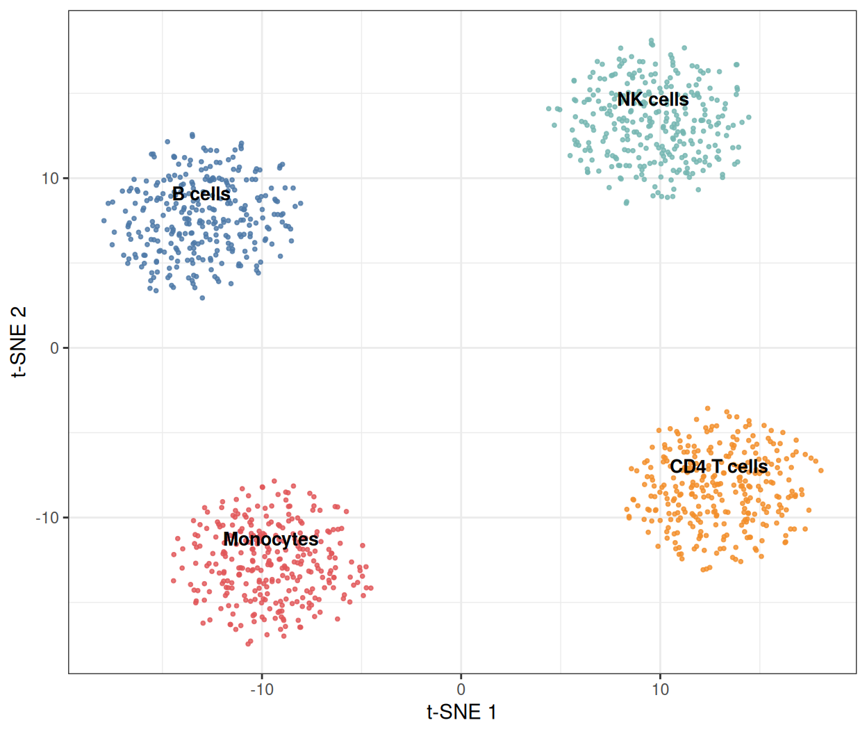

图 1: 模拟队列的 t-SNE 地图（perplexity 30）：四个群体分离为岛屿；标签位于簇质心。

四个岛屿对应四个群体。注意坐标轴：t-SNE 维度没有单位和固定方向——换一个种子重跑，地图会旋转或镜像，但邻域结构保持不变。

2. 困惑度的权衡

perplexity（粗略地说，每个点考虑的”有效邻居数”）是影响最大的单一参数。低值解析局部细节，高值合并群体；数千细胞常用 5–50，诚实的报告应展示图形在一段范围内稳定。

mk <- function(ppl) {
  set.seed(251)
  ts <- Rtsne(pcs, dims = 2, perplexity = ppl, pca = FALSE, verbose = FALSE)
  data.frame(tSNE1 = ts$Y[, 1], tSNE2 = ts$Y[, 2], celltype = ct, perplexity = ppl)
}
dfp <- bind_rows(mk(5), mk(30), mk(100))

ggplot(dfp, aes(tSNE1, tSNE2, color = celltype)) +
  geom_point(size = 0.6, alpha = 0.8) +
  facet_wrap(~perplexity, labeller = labeller(
    perplexity = function(x) paste0("perplexity = ", x))) +
  scale_color_manual(values = pal) +
  labs(x = "t-SNE 1", y = "t-SNE 2") +
  theme_bw(base_size = 11) +
  theme(legend.position = "bottom")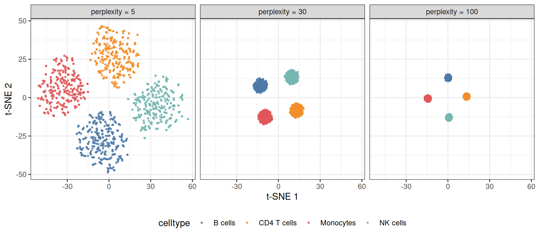

图 2: 同一数据在 perplexity 5、30、100 下的嵌入：低值把群体碎裂成亚结构，高值把群体压成团块。

perplexity 为 5 时，标记块的噪声把每个群体碎裂成亚簇；为 100 时四个群体被压成没有结构的团块。解释任何 t-SNE 图时都要把 perplexity 写进图注。

3. t-SNE 与 PCA 对比

pdf <- data.frame(PC1 = pcs[, 1], PC2 = pcs[, 2], celltype = ct)
p3a <- ggplot(pdf, aes(PC1, PC2, color = celltype)) +
  geom_point(size = 0.6, alpha = 0.8) +
  scale_color_manual(values = pal) +
  labs(x = "PC 1", y = "PC 2", title = "PCA (linear)") +
  theme_bw(base_size = 11) + theme(legend.position = "none")
p3b <- p1 + labs(title = "t-SNE (nonlinear)")

p3a / p3b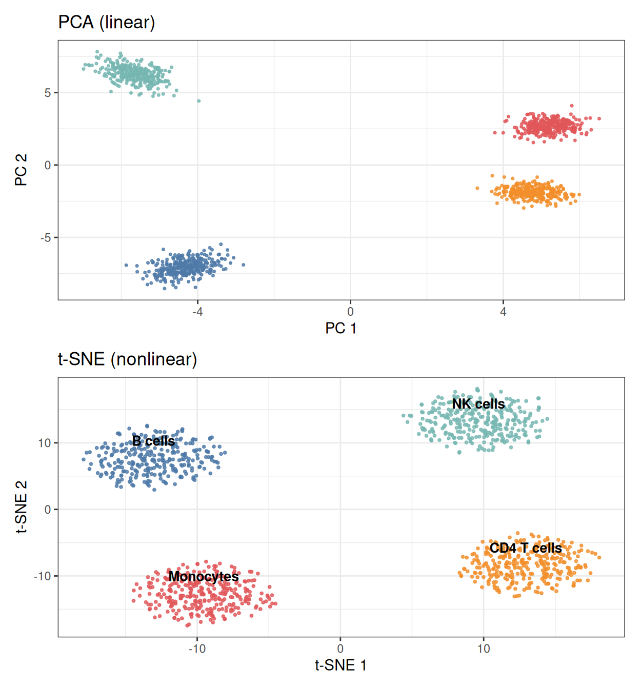

图 3: PCA（上）保留全局几何与相对大小；t-SNE（下）隔离群体但丢弃全局距离。

PCA 保留群体的真实相对大小与位置；t-SNE 均衡簇面积并拉伸空间使邻居贴合。需要量级与梯度信息（轨迹端点、批次偏移）用 PCA，需要发现群体结构用 t-SNE。

4. 叠加标记基因表达

dfm <- d30
dfm$marker <- expr[, "Gene1"]          # CD4 T 细胞标记块成员

ggplot(dfm, aes(tSNE1, tSNE2, color = marker)) +
  geom_point(size = 0.7, alpha = 0.9) +
  scale_color_gradient(low = "#EEEEEE", high = "#B2182B", name = "Gene1") +
  labs(x = "t-SNE 1", y = "t-SNE 2") +
  theme_bw(base_size = 11)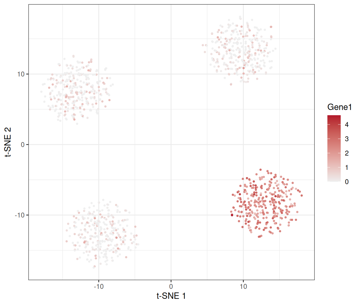

图 4: 把 CD4 T 细胞标记基因（Gene1）的表达画在 t-SNE 地图上：梯度证实了岛屿的身份。

把每细胞数值（基因表达、打分、QC 指标）画上地图，正是 t-SNE 图获得解释力的方式。

实践要点

Rtsne() 之前务必 set.seed()——优化过程是随机的，不设种子的地图不可复现。
输入前 20–50 个 PC 而非原始特征：先去噪是”结构”与”噪声”的分界（还快得多）。
报告 perplexity；在至少两个取值下确认簇边界再下结论。
切勿解读全局距离：地图上相距很远的两个岛屿未必比相邻的两个”差异更大”。
t-SNE 无法把新样本嵌入已有地图——需要增量嵌入用 UMAP，否则只能重新拟合。

Application

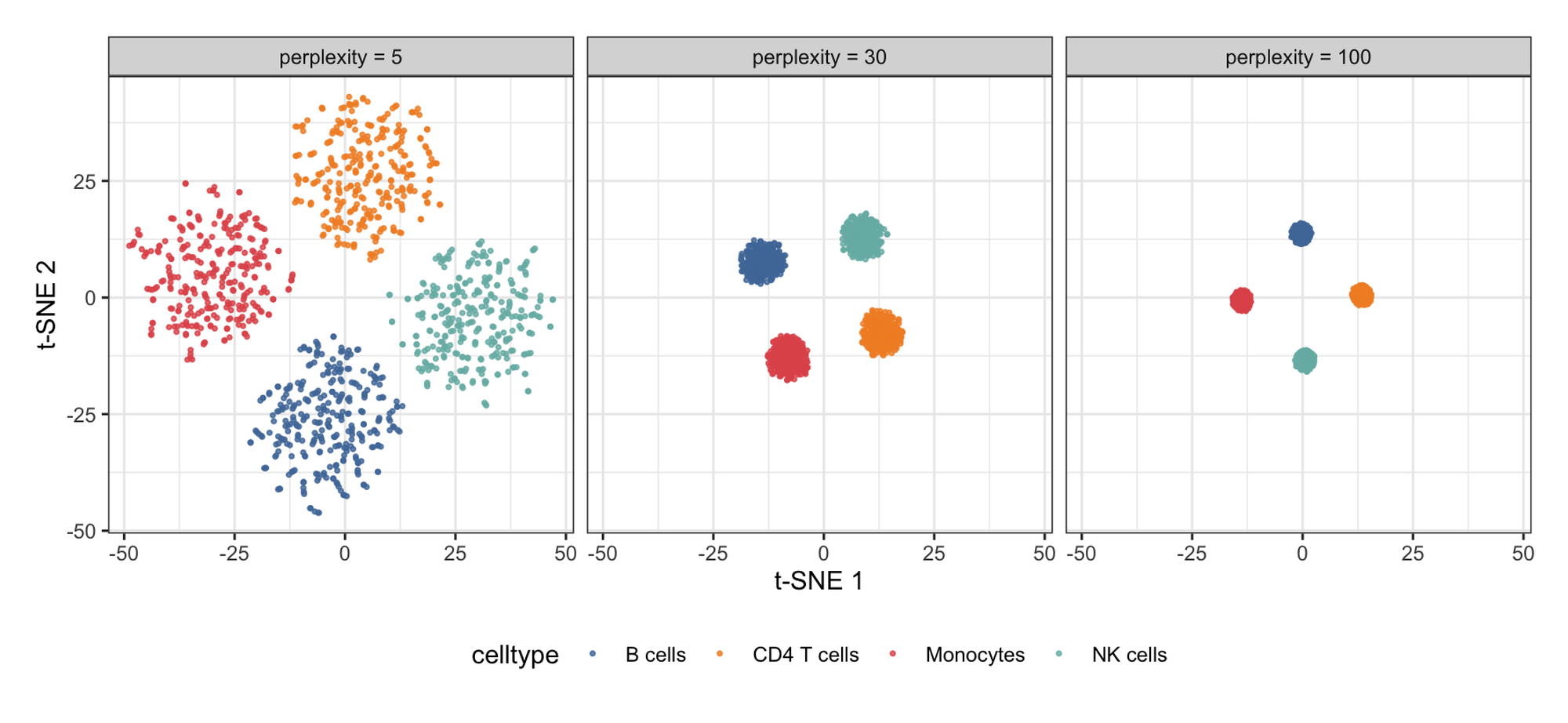
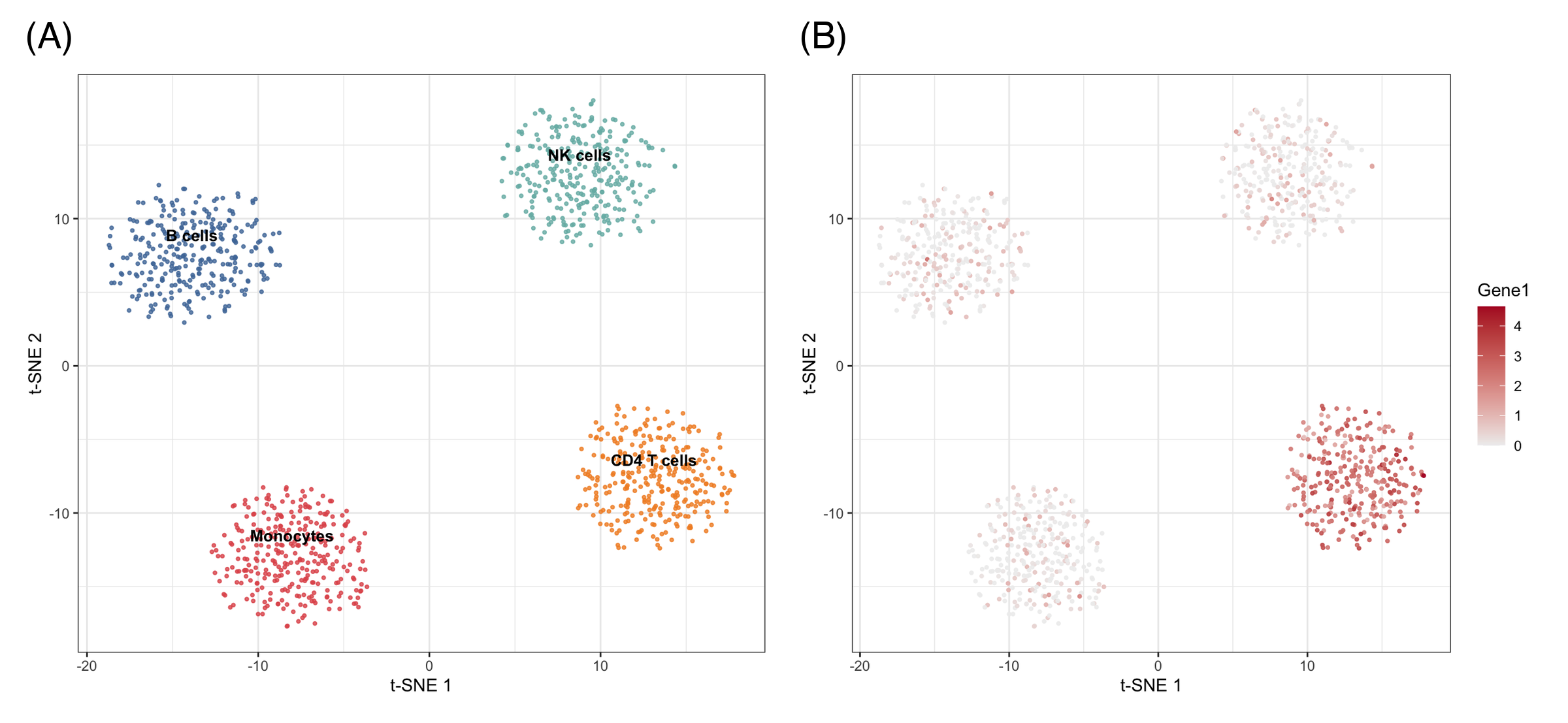
t-SNE 地图是单细胞论文的门面图（细胞类型图谱、肿瘤免疫浸润），凡需把大量特征压缩为群体地图的场景均适用：流式细胞面板、甲基化谱、药物筛选形态学。下图模拟典型论文版式：(A) 困惑度检查与 (B) 带标记叠加的群体地图。

Reference

[1] van der Maaten L, Hinton G. Visualizing data using t-SNE. J Mach Learn Res. 2008;9:2579-2605.

[2] Kobak D, Berens P. The art of using t-SNE for single-cell transcriptomics. Nat Commun. 2019;10:5416. doi:10.1038/s41467-019-13056-x

[3] Krijthe JH. Rtsne: t-Distributed Stochastic Neighbor Embedding using Barnes-Hut implementation. R package version 0.17. 2015. https://github.com/jkrijthe/Rtsne