# 安装包
if (!requireNamespace("streamgraph", quietly = TRUE)) {
  remotes::install_github("hrbrmstr/streamgraph")
}
if (!requireNamespace("dplyr", quietly = TRUE)) {
  install.packages("dplyr")
}
if (!requireNamespace("htmlwidgets", quietly = TRUE)) {
  install.packages("htmlwidgets")
}
if (!requireNamespace("ggplot2", quietly = TRUE)) {
  install.packages("ggplot2")
}
if (!requireNamespace("ggstream", quietly = TRUE)) {
  install.packages("ggstream")
}

# 加载包
library(streamgraph)
library(dplyr)
library(htmlwidgets)
library(ggplot2)
library(ggstream)流线图
流线图是一种堆叠区域图。它表示多个群体的数字变量的演变。通常在中心轴周围显示区域,边缘呈圆弧状以形成流动的形状。
示例
环境配置
系统要求: 跨平台(Linux/MacOS/Windows)
编程语言:R
依赖包:
streamgraph,dplyr,htmlwidgets,ggplot2,ggstream
sessioninfo::session_info("attached")─ Session info ───────────────────────────────────────────────────────────────
setting value
version R version 4.6.0 (2026-04-24)
os Ubuntu 24.04.4 LTS
system x86_64, linux-gnu
ui X11
language (EN)
collate C.UTF-8
ctype C.UTF-8
tz UTC
date 2026-05-09
pandoc 3.1.3 @ /usr/bin/ (via rmarkdown)
quarto 1.9.37 @ /usr/local/bin/quarto
─ Packages ───────────────────────────────────────────────────────────────────
package * version date (UTC) lib source
dplyr * 1.2.1 2026-04-03 [1] RSPM
ggplot2 * 4.0.3.9000 2026-05-04 [1] Github (tidyverse/ggplot2@6870419)
ggstream * 0.1.0 2026-05-04 [1] Github (davidsjoberg/ggstream@a64b8d0)
htmlwidgets * 1.6.4 2023-12-06 [1] RSPM
streamgraph * 0.9.0 2026-05-04 [1] Github (hrbrmstr/streamgraph@76f7173)
[1] /home/runner/work/_temp/Library
[2] /opt/R/4.6.0/lib/R/site-library
[3] /opt/R/4.6.0/lib/R/library
* ── Packages attached to the search path.
──────────────────────────────────────────────────────────────────────────────数据准备
主要运用R内置数据集ChickWeight和一批2020年新冠感染的数据。
# 1.R内置的data——ChickWeight
## 此样本一共有50个样本,下面的数据集chick_new_2 选择了Diet为1的5个代表性样本
chick_new_1 <- subset(ChickWeight,Diet=="1")
chick_new_2 <- chick_new_1[c(1:12,144:155,73:95,156:167),]

# 2.2020年新冠病毒感染的数据(数据来源于GISAID数据库)
## 通过数据整理得到以下数据,covid_all表示每个月内不同地区感染新冠肺炎病毒的总人数
covid_all <- readr::read_csv(
"https://bizard-1301043367.cos.ap-guangzhou.myqcloud.com/covid_all.csv")
head(covid_all)
# A tibble: 6 × 6
...1 X.1 X location time count
<dbl> <dbl> <dbl> <chr> <date> <dbl>
1 1 1 1 Africa 2020-01-01 17
2 2 2 2 Asia 2020-01-01 787
3 3 3 3 Europe 2020-01-01 119
4 4 4 4 North America 2020-01-01 78
5 5 5 5 South America 2020-01-01 2
6 6 6 6 Africa 2020-02-01 14covid_month <- readr::read_csv(
"https://bizard-1301043367.cos.ap-guangzhou.myqcloud.com/covid_month.csv")
head(covid_month)# A tibble: 6 × 7
...1 X.2 X.1 X location month count
<dbl> <dbl> <dbl> <dbl> <chr> <dbl> <dbl>
1 1 1 1 1 Africa 1 17
2 2 2 2 2 Asia 1 787
3 3 3 3 3 Europe 1 119
4 4 4 4 4 North America 1 78
5 5 5 5 5 South America 1 2
6 6 6 6 6 Africa 2 14可视化
1. 基本绘图(运用streamgraph包)
可以用简单的几行代码构建流线图。
1.1 基本代码
以2020年新冠病毒感染的数据为例
streamgraph(covid_all, key = "location",
            value = "count",date = "time",
            height="300px", width="1000px")
基本绘图
这个流线图描述了不同地区在2020年不同时间段感染新冠病毒的人数。
运用streamgraph包创作的流线图,可直接将鼠标放在不同颜色上,图形会直接显示具体信息;也可以通过下拉按钮知道每个样本的具体情况。
1.2 添加下拉按钮
通过sg_legend()函数,添加下拉按钮。与其他streamgraph()选项不同,sg_legend()是在管道命令(%>%)之后使用的。
streamgraph(covid_all, key = "location",
            value = "count",date = "time",
            height="300px", width="1000px") %>%
  sg_legend(show=TRUE, label="location: ")
添加下拉按钮
1.3 改变形状
可通过调整interpolate参数改变流线图形状
streamgraph(covid_all, key = "location",
            value = "count",date = "time",
            interpolate="step",
            height="300px", width="1000px") %>%
sg_legend(show=TRUE, label="location: ")
改变形状
这个流线图描述了不同地区在2020年不同时间段感染新冠病毒的人数。
1.4 改变颜色
scale_fill_brewer():使用一个 R ColorBrewer调色板,包括连续和分类的。scale_fill_manual():构建自定义颜色调色板:只需提供一个包含所选颜色的向量即可。
streamgraph(covid_all,key = "location",
            value = "count",date = "time",
            interpolate="linear",
            height="300px", width="1000px") %>%
  sg_fill_brewer("Reds")
改变颜色
这个流线图描述了不同地区在2020年不同时间段感染新冠病毒的人数。
2. 流线图的偏移
有以下三种情况:
-
silhouette: 形状显示在水平轴的两侧 -
zero: 显示在0线之上。 -
expand: 相当于百分比堆积面积图,完整高度用于可视化百分比。
2.1 silhouette
streamgraph(covid_all,key = "location",
            value = "count",date = "time",
            offset="silhouette",
            height="300px", width="1000px")
silhouette
这个流线图描述了不同地区在2020年不同时间段感染新冠病毒的人数。
2.2 zero
streamgraph(covid_all,key = "location",
            value = "count",date = "time",
            offset="zero",
            height="300px", width="1000px")
zero
这个流线图描述了不同地区在2020年不同时间段感染新冠病毒的人数。
2.3 expand
streamgraph(covid_all,key = "location",
            value = "count",date = "time",
            offset="expand",
            height="300px", width="1000px")
expand
这个流线图描述了不同地区在2020年不同时间段感染新冠病毒的人数。
3. 将图表保存为html文件
使用htmlwidgets包的saveWidget()函数
pp <- streamgraph(chick_new,key = "Chick",
                  value = "weight",date = "Time",
                  height="300px", width="1000px")
saveWidget(pp, file=paste0( getwd(), "/HtmlWidget/streamgraphDropdown.html"))
4. 基本绘图(运用ggplot2包)
与streamgraph包相比,ggplot2包可以自定义更加详细的内容。
4.1 基本代码
以2020年新冠病毒感染的数据为例。
covid_all %>%
  ggplot(aes(time, count, fill = location, label = location, color = location)) +
  geom_area()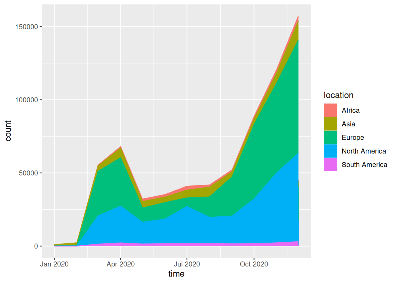
这个流线图描述了不同地区在2020年不同时间段感染新冠病毒的人数。
4.2 美化图形
- 调整曲线形状:
geom_stream() - 调整颜色:
scale_fill_manual()和scale_color_manual()
covid_all %>%
  ggplot(aes(time, count, fill = location, label = location, color = location))  +
geom_stream(type = "ridge", bw=1) 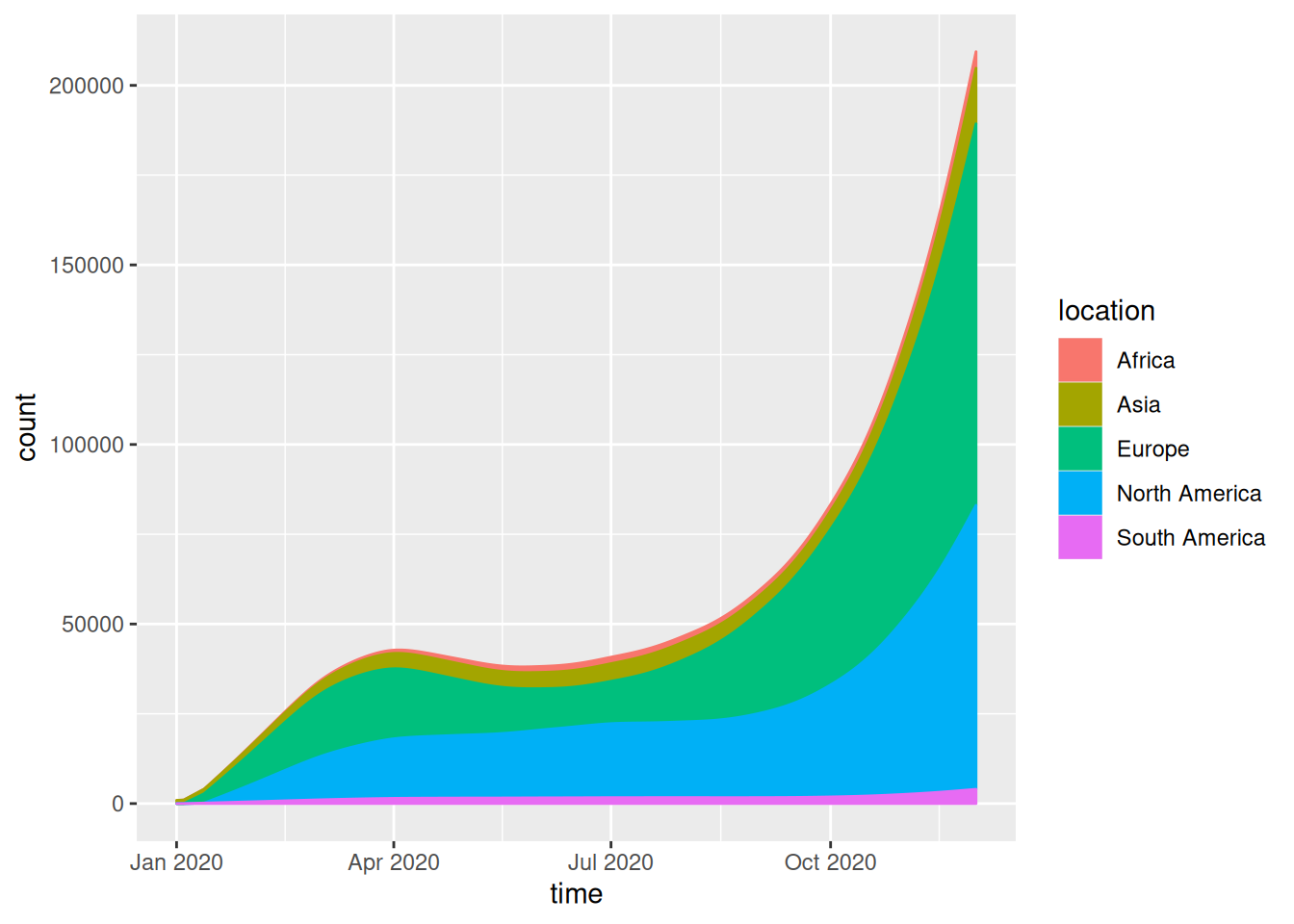
这个流线图描述了不同地区在2020年不同时间段感染新冠病毒的人数。
4.3 以ChickWeight数据为例
chick_new_2 %>%
  ggplot(aes(Time, weight, fill = Chick, label = Chick, color = Chick)) +
  geom_area()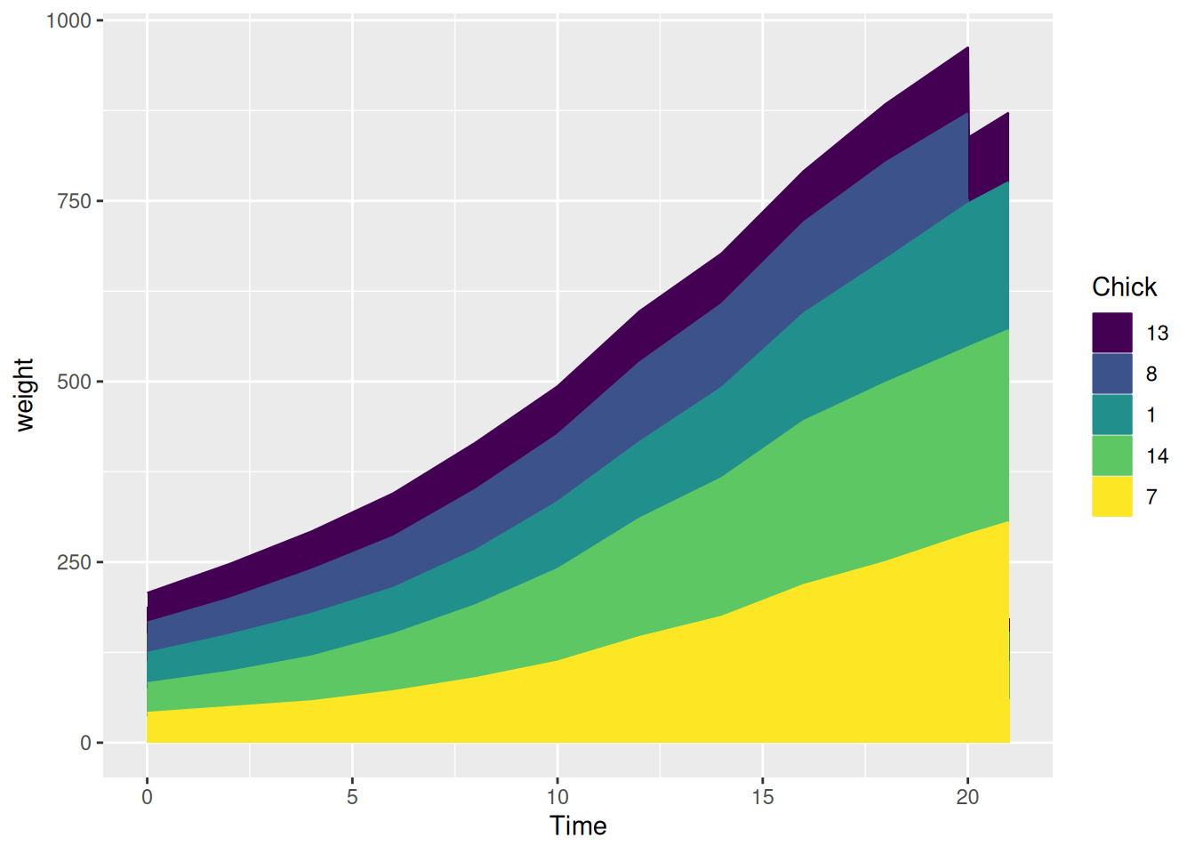
这个流线图描述了不同小鸡体重随时间的变化情况。
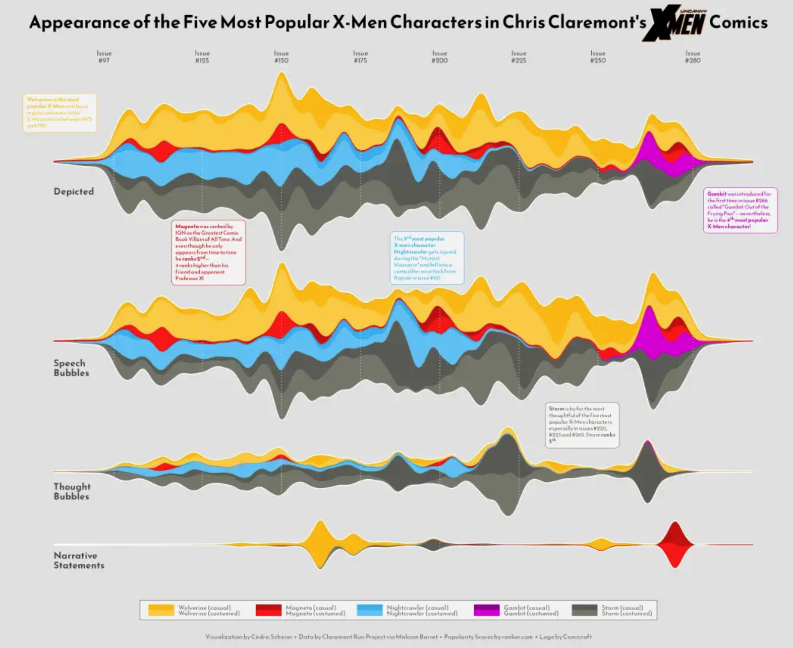
应用场景
这个流线图显示了流感谱系循环的时间变化。 [1]
参考文献
[1] Dhanasekaran V, Sullivan S, Edwards KM, Xie R, Khvorov A, Valkenburg SA, Cowling BJ, Barr IG. Human seasonal influenza under COVID-19 and the potential consequences of influenza lineage elimination. Nat Commun. 2022 Mar 31;13(1):1721. doi: 10.1038/s41467-022-29402-5. PMID: 35361789; PMCID: PMC8971476.
[2] Wickham, H., & François, R. (2019). dplyr: A Grammar of Data Manipulation (Version x.y.z). Retrieved from https://CRAN.R-project.org/package=dplyr
[3] Rudis, B. (2015). streamgraph: An htmlwidget for building streamgraph visualizations. Retrieved from https://github.com/hrbrmstr/streamgraph
[4] Wickham, H., & Romain François. (2024). devtools: Tools to Make Developing R Packages Easier (Version 2.4.5). Retrieved from [https://CRAN.R-project.org/package=devtools](https://cran.r-project.org/package=devtools
[5] Vaidyanathan R, Cheng J, Allaire JJ, Xie Y. htmlwidgets: HTML Widgets for R. R package version 1.6.4. 2023. Available from: https://CRAN.R-project.org/package=htmlwidgets.
[6] David Sjoberg (2021). ggstream: Create Streamplots in ‘ggplot2’. R package version 0.1.0. https://CRAN.R-project.org/package=ggstream